The mean values

1.

1

2. Part 1 THE MEAN VALUES

2

3. СHAPTER QUESTIONS

1. Measures of location
2. Types of means
3. Measures of location for ungrouped data
- Arithmetic mean
- Harmonic mean
- Geometric mean
- Median and Mode
4. Measures of location for grouped data
- Arithmetic mean
- Harmonic mean
- Geometric mean
- Median and Mode
3

4.

• Properties to describe numerical data:
– Central tendency
– Dispersion
– Shape
• Measures calculated for:
– Sample data
• Statistics
– Entire population
• Parameters
4

5.

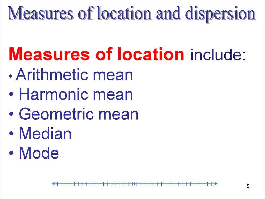
Measures of location include:
• Arithmetic
mean
• Harmonic mean
• Geometric mean
• Median
• Mode
5

6.

UNGROUPED or raw data refers to data as
they were collected, that is, before they are
summarised or organised in any way or form
GROUPED data refers to data summarised in
a frequency table
6

7. What is the mean?

• The mean - is a general
indicator characterizing the
typical level of varying trait
per unit of qualitatively
homogeneous population.
7

8.

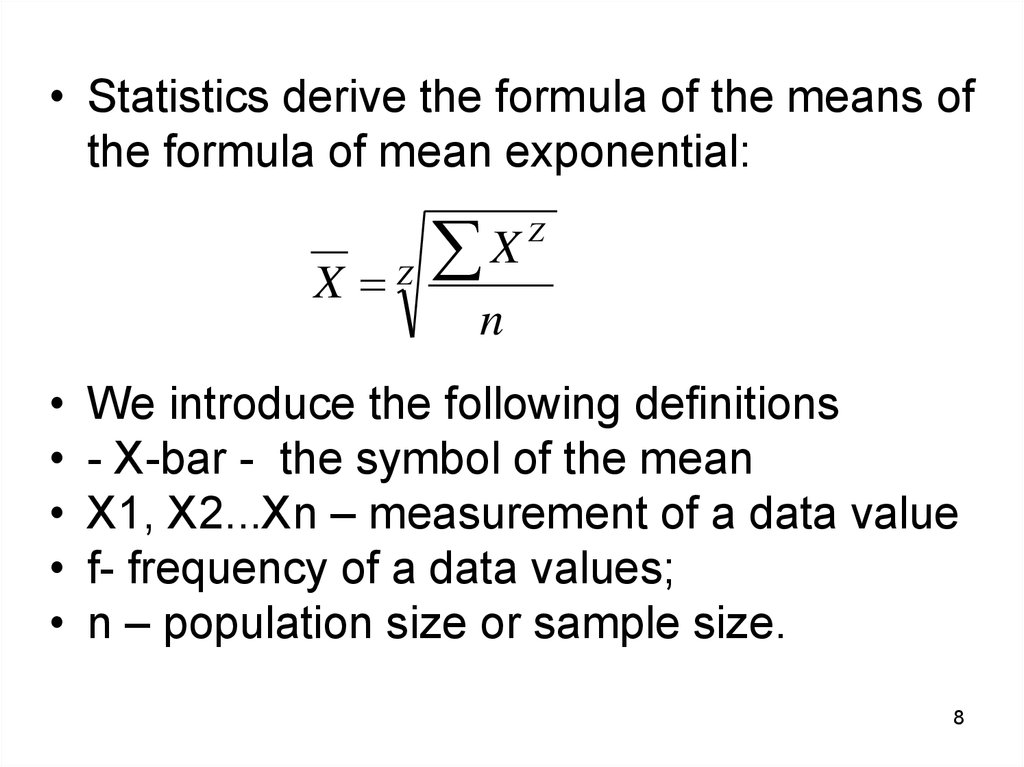
• Statistics derive the formula of the means of
the formula of mean exponential:
X Z
X
Z
n
We introduce the following definitions
- X-bar - the symbol of the mean
Х1, Х2...Хn – measurement of a data value
f- frequency of a data values​​;
n – population size or sample size.
8

9.

• There are the following types of
mean:
• If z = -1 - the harmonic mean,
• z = 0 - the geometric mean,
• z = +1 - arithmetic mean,
• z = +2 - mean square,
• z = +3 - mean cubic, etc.
9

10.

• The higher the degree of z, the greater the
value of the mean. If the characteristic
values ​are equal, the mean is equal to this
constant.
• There is the following relation, called the
rule the majorizing mean:
x harm x geom x arith x sq
10

11.

There are two ways of
calculating mean:
• for ungrouped data is calculated as a simple mean
• for grouped data is calculated weighted mean
11

12. Types of means

Mean
Formula
for ungrouped data simple
Harmonic
mean
x
(xf = M)
Geometric
mean
Arithmetic
mean
n
1
x
i
x П ( xi )
n
x
xi
n
for grouped data –
weighted
M
x
M
x
i
i
i
fi
fi
x
П ( xi )
xf
x
f
i i
i

13. Arithmetic mean

Arithmetic mean value is
called the mean value of the
sign, in the calculation of the
total volume of which feature
in the aggregate remains
unchanged
13

14. Characteristics of the arithmetic mean

The arithmetic mean has a number of
mathematical properties that can be used to
calculate it in a simplified way.
1. If the data values (Xi) to reduce or increase
by a constant number (A), the mean,
respectively, decrease or increase by a
same constant number (A)
( x A) f
f
i
i
i
x f
f
i
i
i
A f i
f
i
x A
14

15.

• 2. If the data values (Xi) divided or multiplied
by a constant number (A), the mean
decrease or increase, respectively, in the
same amount of time (this feature allows you
to change the frequency of specific gravities relative frequency):
• a) when divided by a constant number:
xi
1
f
A i A xi f i 1 x
x
fi
fi A A
• b) when multiplied by a constant number:
xAf
f
i
i
A xi f i
f
i
A x
15

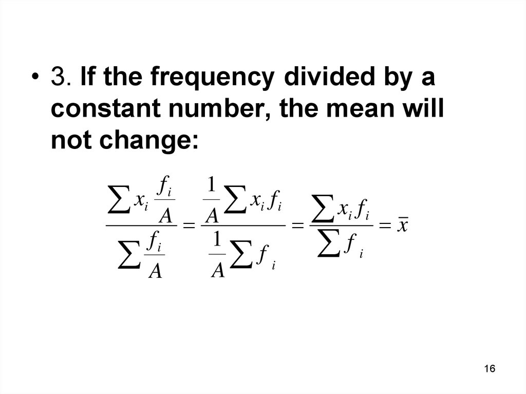
16.

• 3. If the frequency divided by a
constant number, the mean will
not change:
fi
xi A
fi
A
1
xi f i
A
1
fi
A
x f
f
i
i
x
i
16

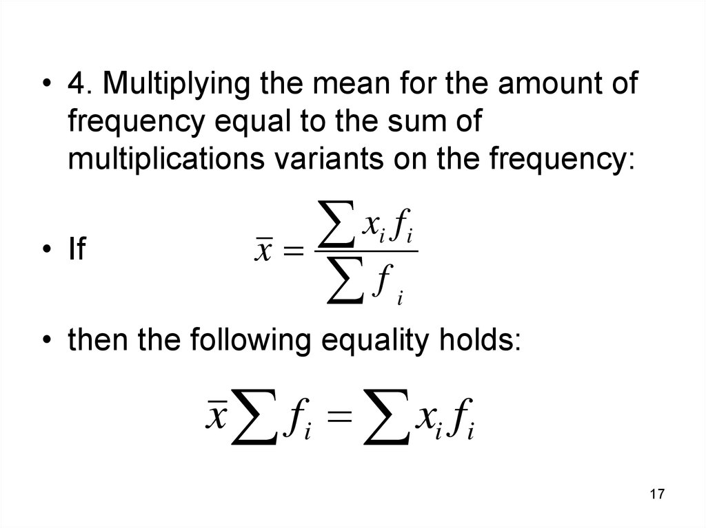
17.

• 4. Multiplying the mean for the amount of
frequency equal to the sum of
multiplications variants on the frequency:
• If
xf
x
f
i i
i
• then the following equality holds:
x fi xi fi
17

18.

5.The sum of the deviations of the
number in a data value from the
mean is zero:
(x x) 0
i
• If xi f i x f i
• then xi f i x f i 0
• So xi f i x f i ( xi x ) f i 0
18

19. Measures of location for ungrouped data

• In calculating summary values for a data
collection, the best is to find a central, or
typical, value for the data.
• More important measures of central
tendency are presented in this section:
• Mean (simple or weighter)
• Median and Mode
19

20.

ARITHMETIC MEAN
- This is the most commonly used measure.
- The arithmetic mean is a summary value
calculated by summing the numerical data
values and dividing by the number of values
sum of sample observations
Sample mean =
number of sample observations
n
x
x
i 1
n
i
Sample size
20

21.

ARITHMETIC MEAN
- This is the most commonly used measure and
is also called the mean.
sum of observations
Population mean =
number of observations
N
Mean
xi
i 1
N
Xi = observations of the population
∑ = “the sum of”
Population size
21

22. Example - The sales of the six largest restaurant chains are presented in table

Company
McDonald’s
Sales ($ million)
14.110
Burger King
Kentucky Fried Chicken
Hardee’s
5.590
3.700
3.030
Wendy’s
Pizza Hut
2.800
2.450
A mean sales amount of 5.280 $ million is computed
using Equation of arithmetical mean simple
14100 5590 3700 3030 2800 2450
x
5280
22
6

23. MEDIAN for ungrouped data

• The median of a data is the middle item in
a set of observation that are arranged in
order of magnitude.
• The median is the measure of location
most often reported for annual income
and property value data.
• A few extremely large incomes or
property values can inflate the mean.
23

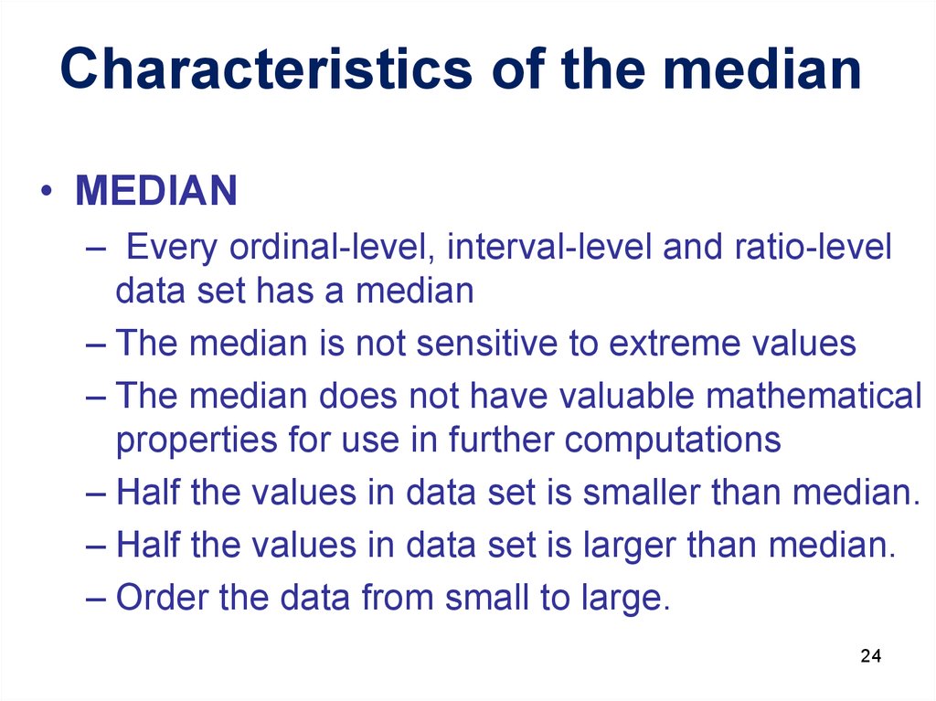
24.

Characteristics of the median
• MEDIAN
– Every ordinal-level, interval-level and ratio-level
data set has a median
– The median is not sensitive to extreme values
– The median does not have valuable mathematical
properties for use in further computations
– Half the values in data set is smaller than median.
– Half the values in data set is larger than median.
– Order the data from small to large.
24

25. Position of median

– If n is odd:
• Median item number = (n+1)/2
– If n is even:
• Calculate (n+1)/2
• The median is the average of the
values before and after (n+1)/2.
25

26. Example

• The median number of people treated daily at the
emergency room of St. Luke’s Hospital must be
determined from the following data for the last six
days:
25, 26, 45, 52, 65, 78
Since the data values are arranged from lowest to
highest, the median be easily found. If the data
values are arranged in a mess, they must rank.
Median item number = (6+1)/2 =3,5
Since the median is item 3,5 in the array, the third
and fourth elements need to be averaged:
(45+52)/2=48,5. Therefore, 48,5 is the median
number of patients treated in hospital emergency
26
room during the six-day period.

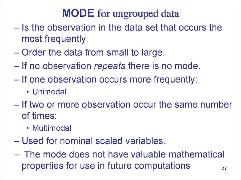
27.

MODE for ungrouped data
– Is the observation in the data set that occurs the
most frequently.
– Order the data from small to large.
– If no observation repeats there is no mode.
– If one observation occurs more frequently:
• Unimodal
– If two or more observation occur the same number
of times:
• Multimodal
– Used for nominal scaled variables.
– The mode does not have valuable mathematical
properties for use in future computations
27

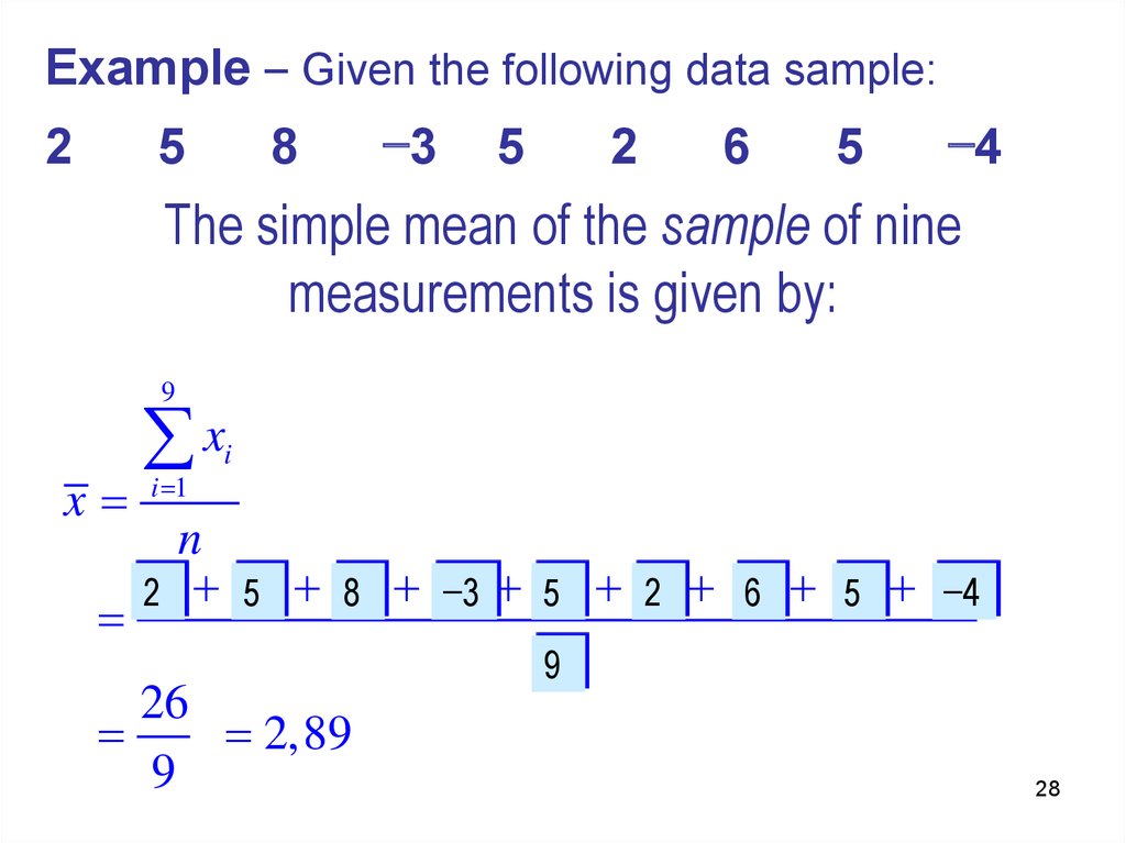
28.

Example – Given the following data sample:
2
5
8
−3
5
2
6
5
−4
The simple mean of the sample of nine
measurements is given by:
9
x
x
i 1
i
n
x21 x52 x83 x−34 x55 x26 x67 x58 x−49
9n
26
2,89
9
28

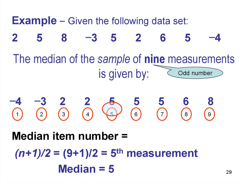
29.

Example – Given the following data set:
2
5
8
−3
5
2
6
5
−4
The median of the sample of nine measurements
Odd number
is given by:
−4
−3
2
2
5
5
5
6
8
1
2
3
4
5
6
7
8
9
Median item number =
(n+1)/2 = (9+1)/2 = 5th measurement
Median = 5
29

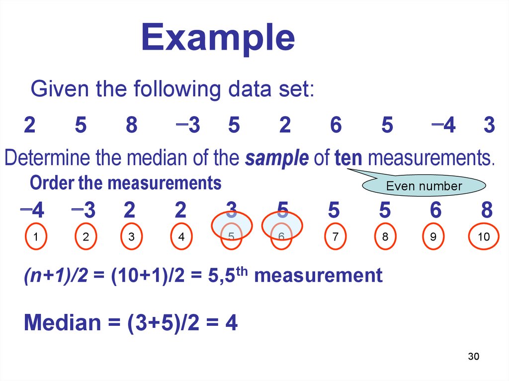
30.

Given the following data set:
2
5
8
−3 5
2
6
5
−4 3
Determine the median of the sample of ten measurements.
Order the measurements
Even number
−4
−3
2
2
3
5
5
5
6
8
1
2
3
4
5
6
7
8
9
10
(n+1)/2 = (10+1)/2 = 5,5th measurement
Median = (3+5)/2 = 4
30

31.

Example
Given the following data set:
2
5
8
−3
5
2
6
5
−4
Determine the mode of the sample of nine measurements.
•Order the measurements
−4
−3
2
2
5
5
5
6
8
Mode = 5
•Unimodal
31

32.

Example
Given the following data set:
2
5
8
−3
5
2
6
5
−4
2
Determine the mode of the sample of ten measurements.
•Order the measurements
−4
−3
2
2
2
5
5
5
6
8
Mode = 2 and 5
•Multimodal - bimodal
32

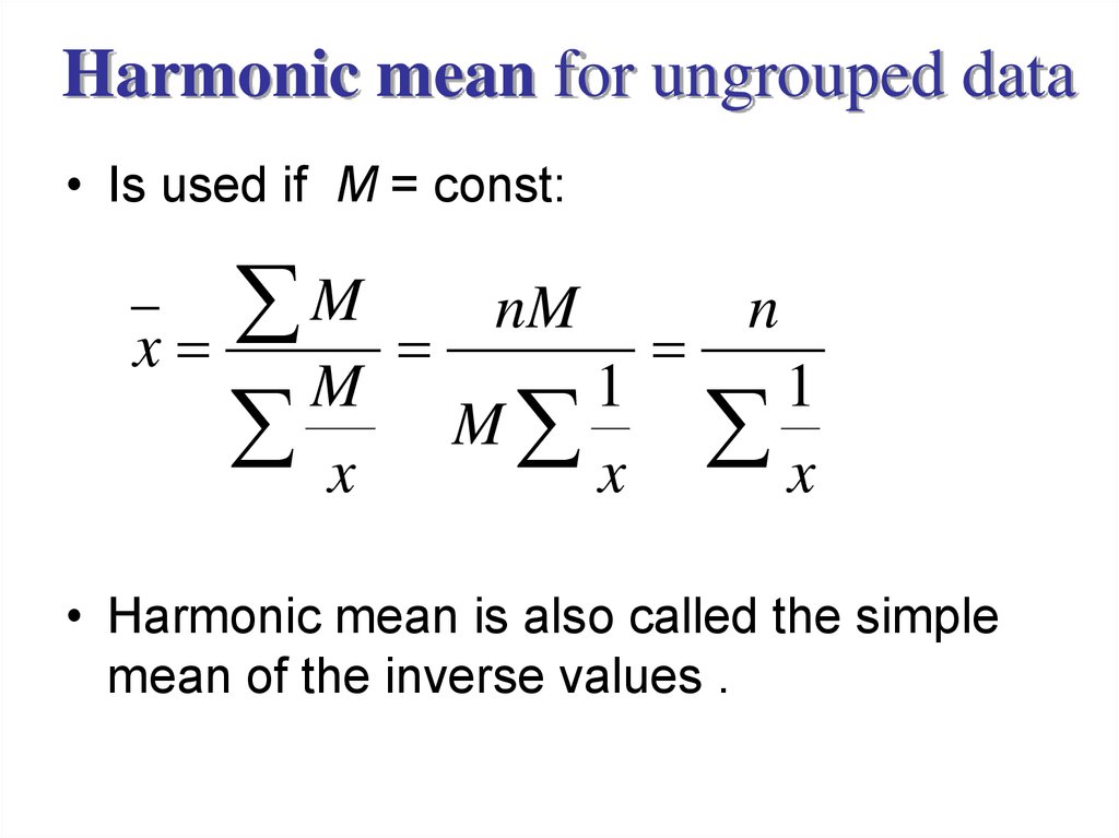
33.

Harmonic mean for ungrouped data
• Is used if М = const:
M
x
M
x
nM
1
M
x
n
1
x
• Harmonic mean is also called the simple
mean of the inverse values .

34.

Harmonic mean for ungrouped data
• For example:
• One student spends on a solution of task
1/3 hours, the second student – ¼
(quarter) and the third student 1/5 hours.
Harmonic mean will be calculated:
1 1 1
3
3 1
x
(hour )
4
1
1
1
1 3 5 4 12
x 1 1 1
3
5
4
n

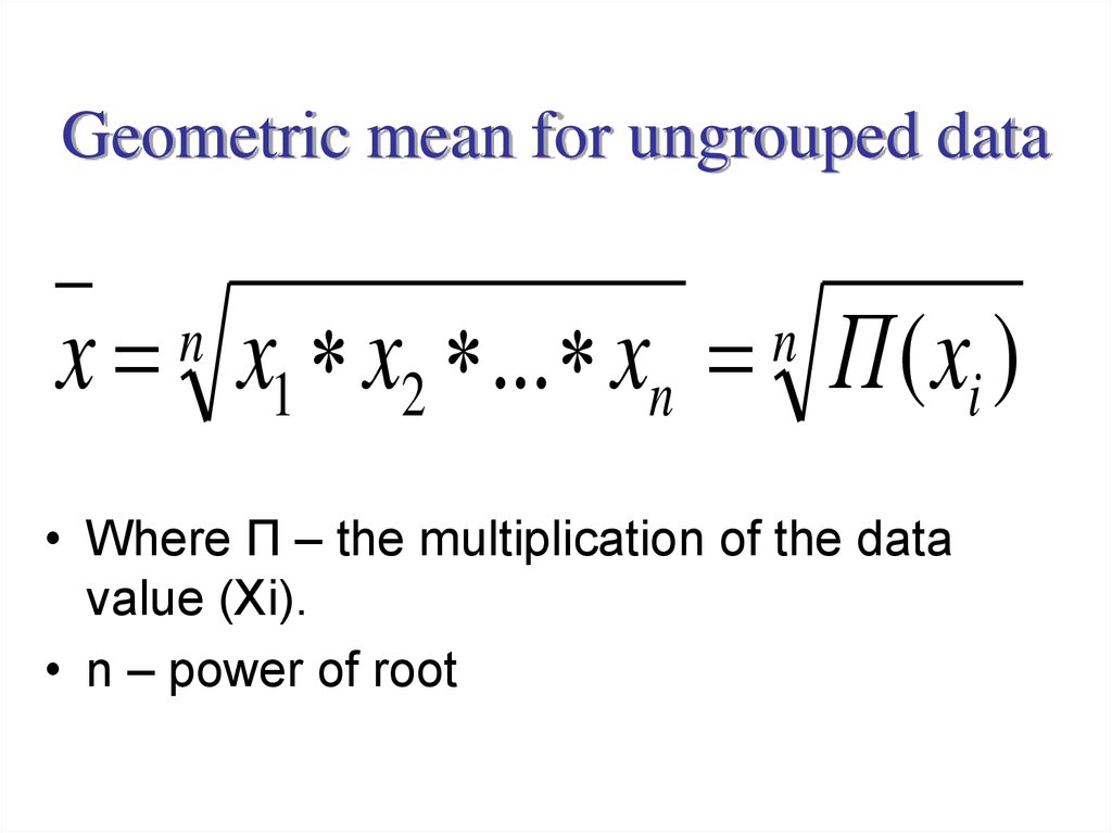
35. Geometric mean for ungrouped data

• This value is used as the
average of the relations between
the two values, or in the ranks of
the distributions presented in the
form of a geometric progression.
35

36.

Geometric mean for ungrouped data
x x1 x2 ... xn П ( xi )
n
n
• Where П – the multiplication of the data
value (Xi).
• n – power of root

37.

Geometric mean for ungrouped data
For example, the known data about the rate
of growth of production
Year
2009
Growth rate 1,24
2010
1,39
2011
1,31
2012
1,15
Calculate the geometric mean. It is 127 percent:
X 1.24 *1.39 *1.31*1.15 1,27
4

38.

• ARITHMETIC MEAN
– Data is given in a frequency table
– Only an approximate value of the mean
fx
x
f
i
i
i
where f i frequency of the i th class interval
xi = class midpoint of the i th class interval
38

39. Example

There are data on seniority hundred
employees in the table
Seniority,
year (х)
The number of
employees (f)
xf
1
9
11
13
15
17
Total
2
10
10
50
20
10
100
3
90
110
650
300
170
1320
39

40.

• Average seniority employee is:
xf
x
f
1320
13,2 year
100
40

41. Harmonic mean for grouped data

• Harmonic mean - is the
reciprocal of the arithmetic
mean. Harmonic mean is used
when statistical information
does not contain frequencies,
and presented as
xf = M.
41

42. Harmonic mean for grouped data

• Harmonic mean is calculated by
the formula:
M
x
M
x
i
i
i
• where M = xf
42

43. Example

There are data on hárvesting the apples by
three teams and on average per worker
Number of
Harvesting the apples, kg
teams
One worker
Whole team
(X)
(M)
1
800
2400
2
1200
9600
3
900
5600
Всего
х
17600
17600
x
1023(kg)
2400 9600 5600
800 1200 900

44.

Geometric mean for grouped data
is calculated by the formula:
fi
fi
x
П ( xi )
fi
f1
f2
f2
( x ) * ( x ) * ... * ( x )
1
2
2
• Where fi – frequency of the data value (Xi)
П – multiplication sign.

45.

Geometric mean for grouped data
EXAMPLE
Year
2010
Growth rate 1,24
2011
1,24
2012
1,31
2013
1,31
Calculate the geometric mean. It is 127,5%
percent:
Х 1.24 2 *1.31 2 1,275
4

46.

• MEDIAN
– Data is given in a frequency table.
– First cumulative frequency ≥ n/2 will indicate the
median class interval.
– Median can also be determined from the ogive.
M e li
ui li n2 Fi 1
where li
ui
Fi -1
fi
fi
= lower boundary of the median interval
= upper boundary of the median interval
= cumulative frequency of interval foregoing
median interval
= frequency of the median interval
46

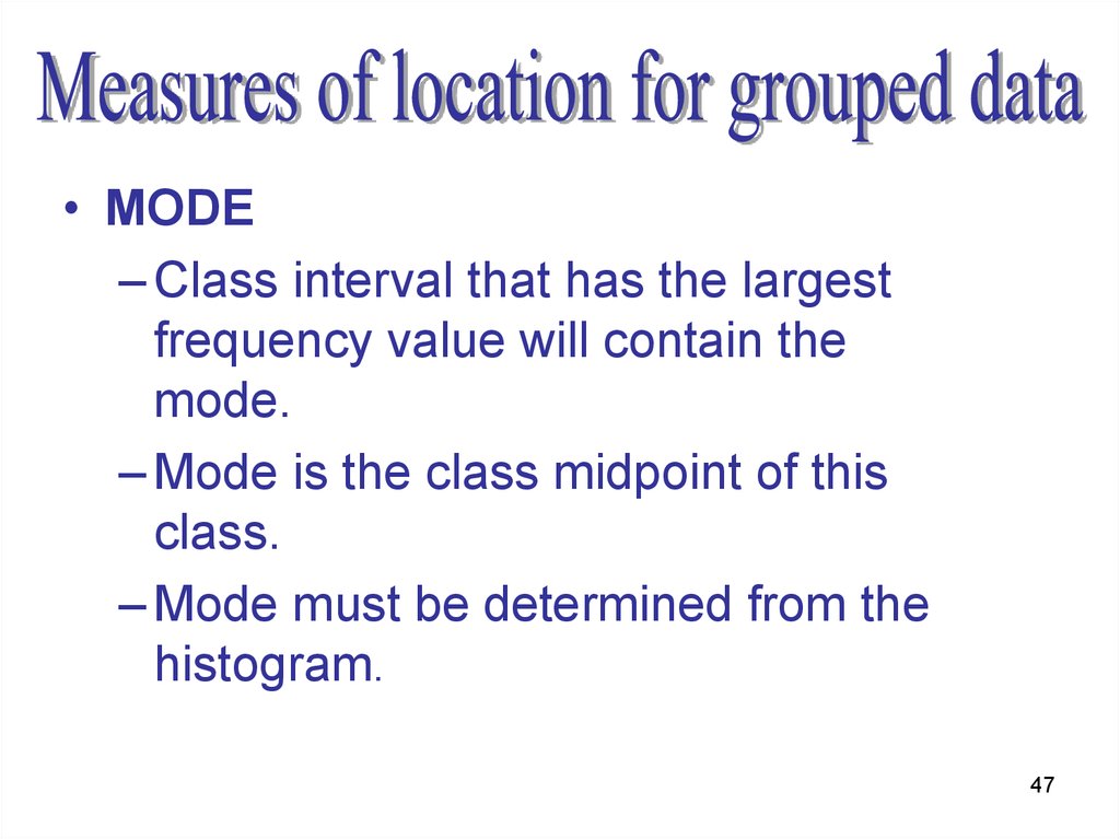
47.

• MODE
– Class interval that has the largest
frequency value will contain the
mode.
– Mode is the class midpoint of this
class.
– Mode must be determined from the
histogram.
47

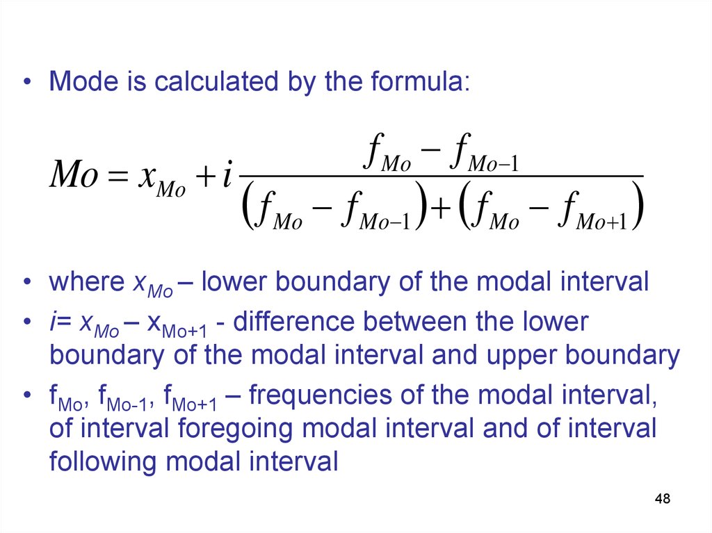
48.

• Mode is calculated by the formula:
f Mo f Mo 1
Mo xMo i
f Mo f Mo 1 f Mo f Mo 1
• where хМо – lower boundary of the modal interval
• i= хМо – xMo+1 - difference between the lower
boundary of the modal interval and upper boundary
• fMo, fMo-1, fMo+1 – frequencies of the modal interval,
of interval foregoing modal interval and of interval
following modal interval
48

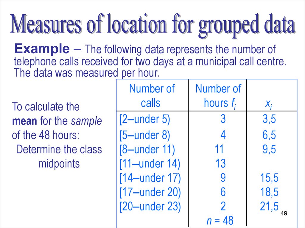
49.

Example – The following data represents the number of
telephone calls received for two days at a municipal call centre.
The data was measured per hour.
Number of
Number of
calls
hours fi
xi
To calculate the
3
3,5
mean for the sample [2–under 5)
[5–under 8)
4
6,5
of the 48 hours:
11
9,5
Determine the class [8–under 11)
[11–under 14)
13
12,5
midpoints
[14–under 17)
9
15,5
[17–under 20)
6
18,5
[20–under 23)
2
21,5 49
n = 48

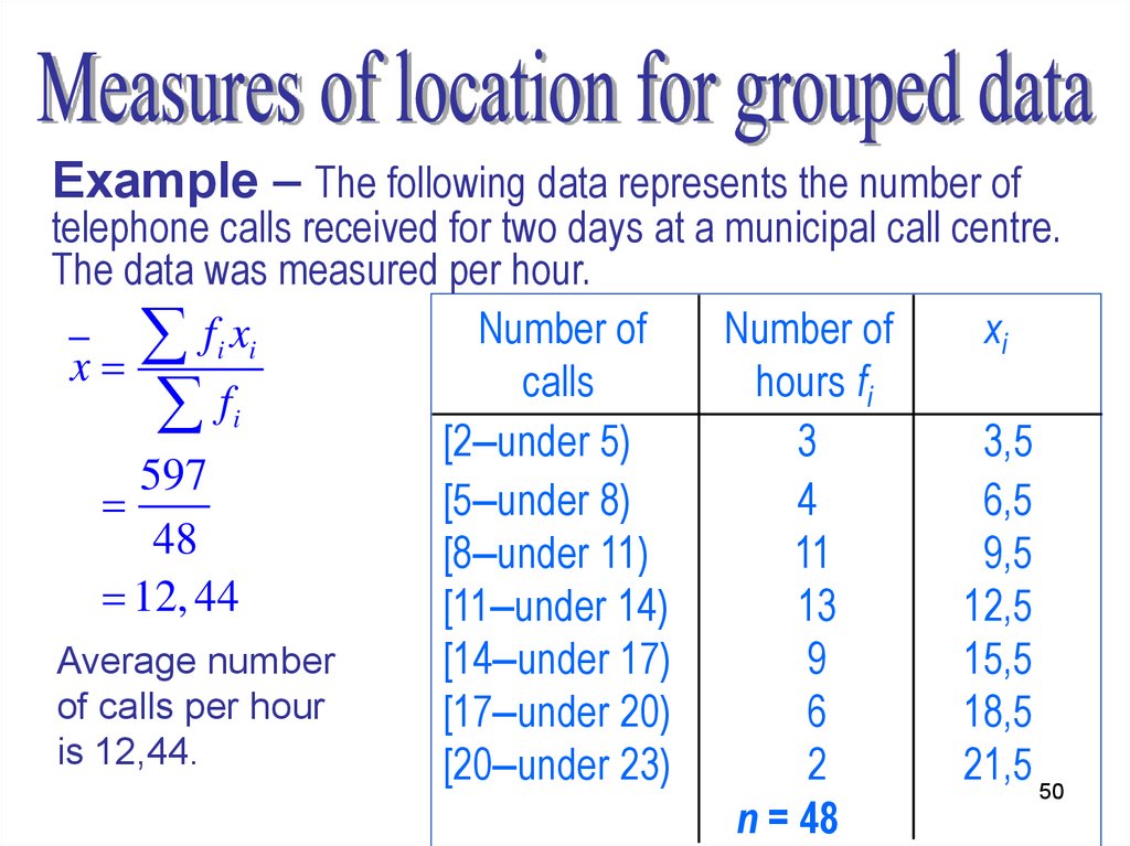
50.

Example – The following data represents the number of
telephone calls received for two days at a municipal call centre.
The data was measured per hour.
Number of
Number of
xi
f i xi
x
calls
hours fi
f
i
[2–under 5)
3
3,5
597
[5–under 8)
4
6,5
48
[8–under 11)
11
9,5
12, 44
[11–under 14)
13
12,5
Average number
[14–under 17)
9
15,5
of calls per hour
[17–under 20)
6
18,5
is 12,44.
[20–under 23)
2
21,5 50
n = 48

51.

Example – The following data represents the number of
telephone calls received for two days at a municipal call centre.
The data was measured per hour.
To calculate the for
Number of
Number of
the sample median
calls
hours fi
F
of the 48: hours:
[2–under 5)
3
3
determine the
[5–under 8)
4
7
cumulative
[8–under 11)
11
18
frequencies
[11–under 14)
13
31
[14–under 17)
9
40
n/2 = 48/2 = 24
[17–under 20)
6
46
The first cumulative
[20–under 23)
2
48 51
frequency ≥ 24
n = 48

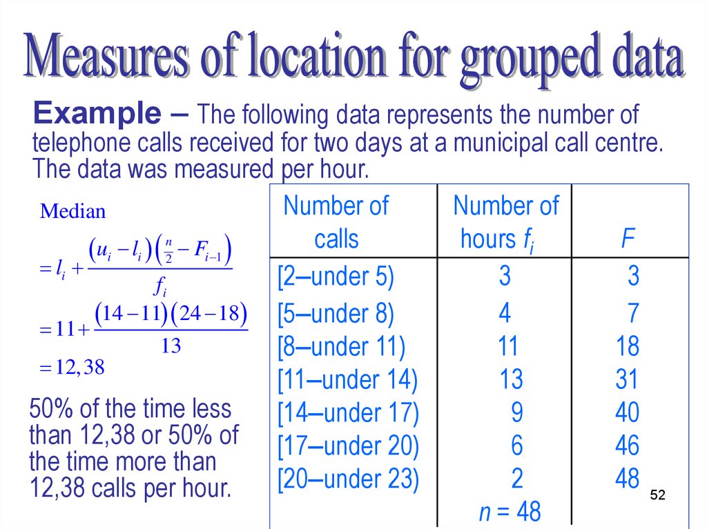
52.

Example – The following data represents the number of
telephone calls received for two days at a municipal call centre.
The data was measured per hour.
Number of
Number of
Median
calls
hours fi
F
ui li n2 Fi 1
li
[2–under 5)
3
3
fi
14 11 24 18 [5–under 8)
4
7
11
13
[8–under 11)
11
18
12,38
[11–under 14)
13
31
50% of the time less
[14–under 17)
9
40
than 12,38 or 50% of [17–under 20)
6
46
the time more than
[20–under 23)
2
48 52
12,38 calls per hour.
n = 48

53.

Example – The following data represents the number of
telephone calls received for two days at a municipal call centre.
The data was measured per hour.
The median can
be determined
form the ogive.
Number of calls at a call centre
Number of hours
48
40
32
n/2 = 48/2 = 24
24
16
8
0
2
5
8
11
A
14
17
20
23
Median = 12,4
Read at A.
Number of calls
53

54.

Example – The following data represents the number of
telephone calls received for two days at a municipal call centre.
The data was measured per hour.
Number of
Number of
calls
hours fi
To calculate the for
the sample mode
[2–under 5)
3
of the 48 hours
[5–under 8)
4
[8–under 11)
11
The modal interval
[11–under 14)
13
[14–under 17)
9
[17–under 20)
6
The highest
[20–under
23)
2
54
frequency
n = 48

55.

MODE
• We substitute the data into the formula:
f Mo f Mo 1
Mo xMo i
f Mo f Mo 1 f Mo f Mo 1
13 11
11 (14 11)
12,3
13 11 13 9
• Mo = 12,3
• So, the most frequent number of calls per
hour = 12.3
55

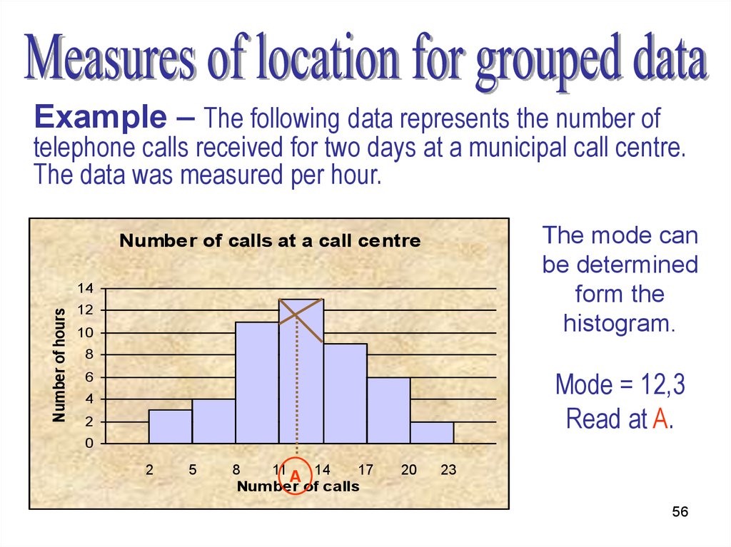
56.

Example – The following data represents the number of
telephone calls received for two days at a municipal call centre.
The data was measured per hour.
The mode can
be determined
form the
histogram.
Number of calls at a call centre
Number of hours
14
12
10
8
Mode = 12,3
Read at A.
6
4
2
0
2
5
8
11
17
A 14
Number of calls
20
23
56

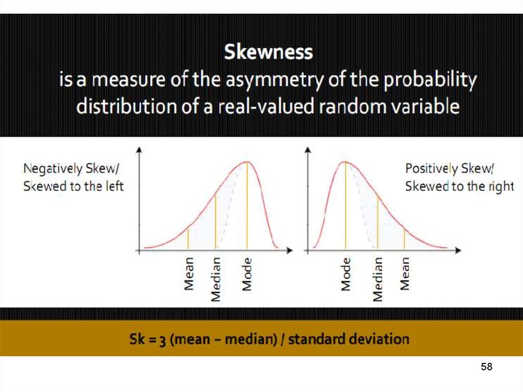
57. Relationship between mean, median, and mode

• If a distribution is symmetrical:
– the mean, median and mode are the same
and lie at centre of distribution
• If a distribution is non-symmetrical:
– skewed to the left or to the right
– three measures differ
A positively skewed distribution
(skewed to the right)
Mode
Mean
Median
Mean
Mode
Median
A negatively skewed distribution
(skewed to the left)
Mean
Mode
Median
57

58.

58

59. EXAMPLE

• Consider a study of the hourly
wage rates in three different
companies, For
simplicity,
assume that they employ the
same number of employees: 100
people.
59

60.

60

61.

• So we have three 100-element
samples, which have the same
average value (35) and the
same variability (120). But these
are different samples. The
diversity of these samples can
be seen even better when we
draw their histograms.
61

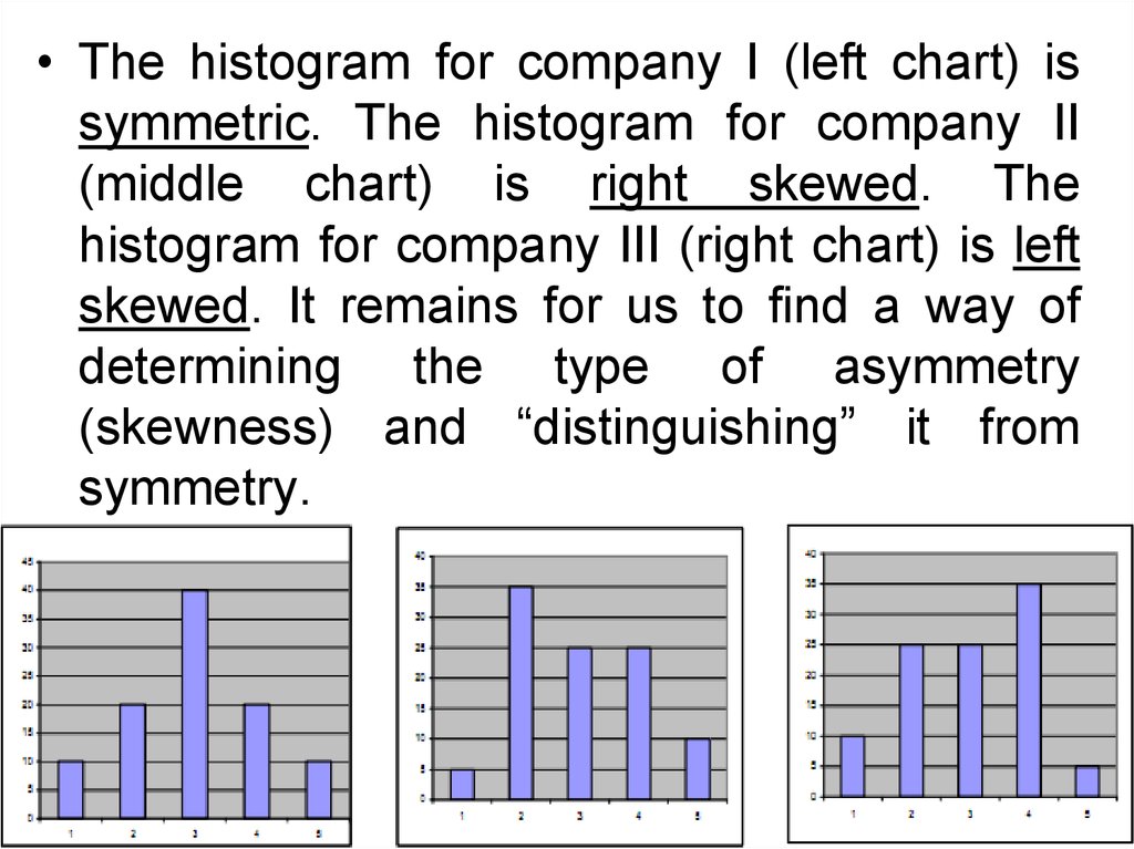
62.

• The histogram for company I (left chart) is
symmetric. The histogram for company II
(middle chart) is right skewed. The
histogram for company III (right chart) is left
skewed. It remains for us to find a way of
determining the type of asymmetry
(skewness) and “distinguishing” it from
symmetry.
62

63.

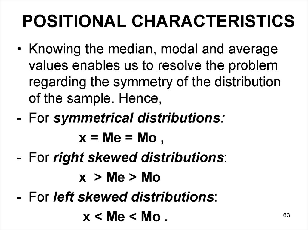
POSITIONAL CHARACTERISTICS
• Knowing the median, modal and average
values enables us to resolve the problem
regarding the symmetry of the distribution
of the sample. Hence,
- For symmetrical distributions:
x = Me = Mo ,
- For right skewed distributions:
x > Me > Mo
- For left skewed distributions:
63
x < Me < Mo .

64.

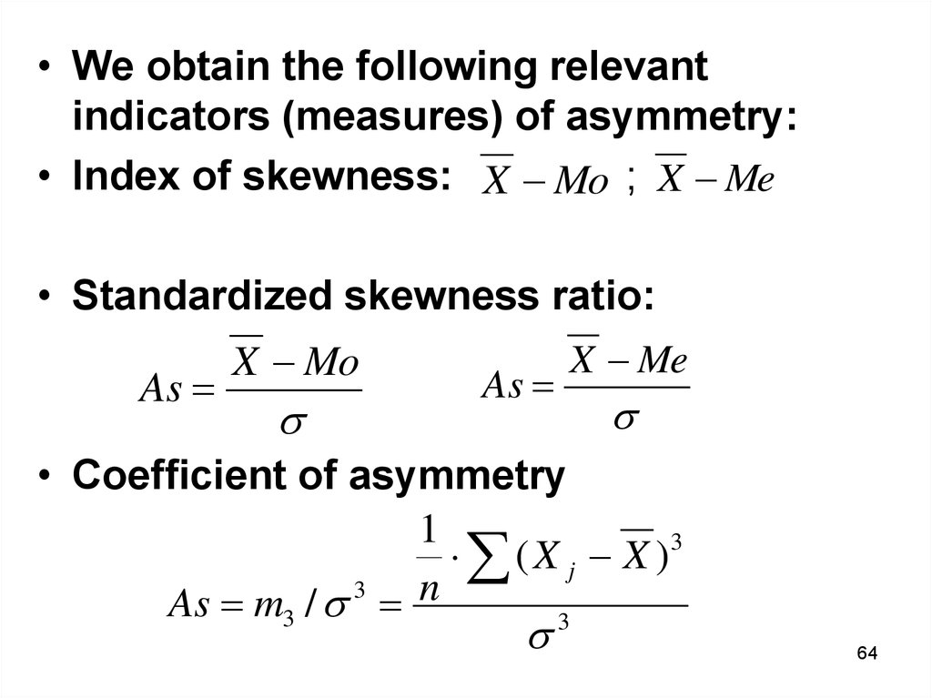
• We obtain the following relevant
indicators (measures) of asymmetry:
• Index of skewness: X Mo ; X Me
• Standardized skewness ratio:
As
X Mo
As
X Me
• Coefficient of asymmetry
1
( X j X )3
As m3 / 3 n
3
64

65. Example

Years Work
of
ers
service (f)
6-10
10-14
14-18
18-22
15
30
45
10
Total: 100
Calculation
Хi
xf
Σf=F x x x x * f x x
x x f
2
2

66.

Years of
service
Workers
(f)
Calculation
Midpoint
xf
Σ f=F
Хi
6-10
10-14
14-18
18-22
15
30
45
10
8
12
16
20
Всего:
100
14
66

67.

Years of
service
Workers
(f)
Calculation
Midpoint
xf
Σ f=F
Хi
6-10
10-14
14-18
18-22
15
30
45
10
8
12
16
20
120
360
720
200
15
45
90
100
Всего:
100
14
1400
x
67

68.

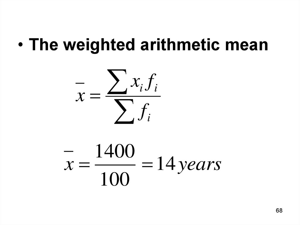
• The weighted arithmetic mean
x f
x
f
i i
i
1400
x
14 years
100
68

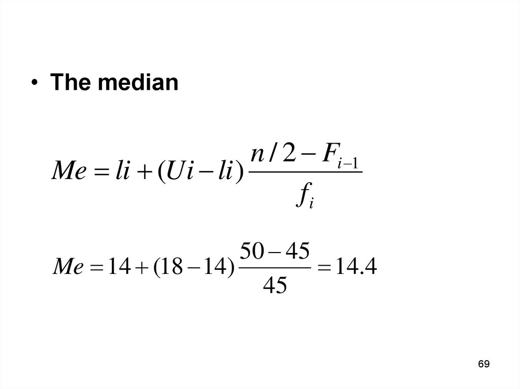
69.

• The median
n / 2 Fi 1
Me li (Ui li )
fi
50 45
Me 14 (18 14)
14.4
45
69

70.

• The mode
f Mo f Mo 1
Mo xMo i
f Mo f Mo 1 f Mo f Mo 1
45 30
Mo 14 (18 14)
15,2
45 30 45 10
70

71.

71