


")


 Механика
Похожие презентации:


")


Motor classification
1. Keywords
Series Wound DC Motor – двигатель постоянного тока споследовательной обмоткой возбуждения
Separately Excited DC Motor – двигатель постоянного тока
независимого возбуждения
permanent-magnet DC motor – двигатель постоянного тока на
постоянных магнитах
Self Excited DC Motor – двигатель с самовозбуждением
Shunt wound DC motor - двигатель с параллельным возбуждением
Compound Wound DC Motor – двигатель смешанного возбуждения
2.
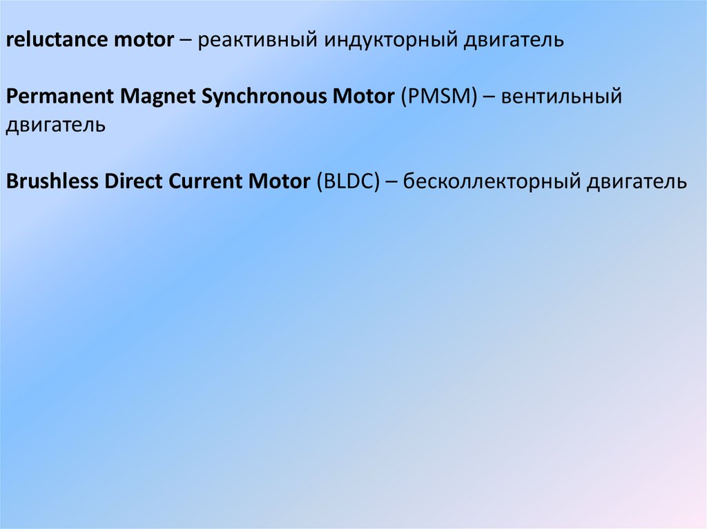
reluctance motor – реактивный индукторный двигательPermanent Magnet Synchronous Motor (PMSM) – вентильный
двигатель
Brushless Direct Current Motor (BLDC) – бесколлекторный двигатель
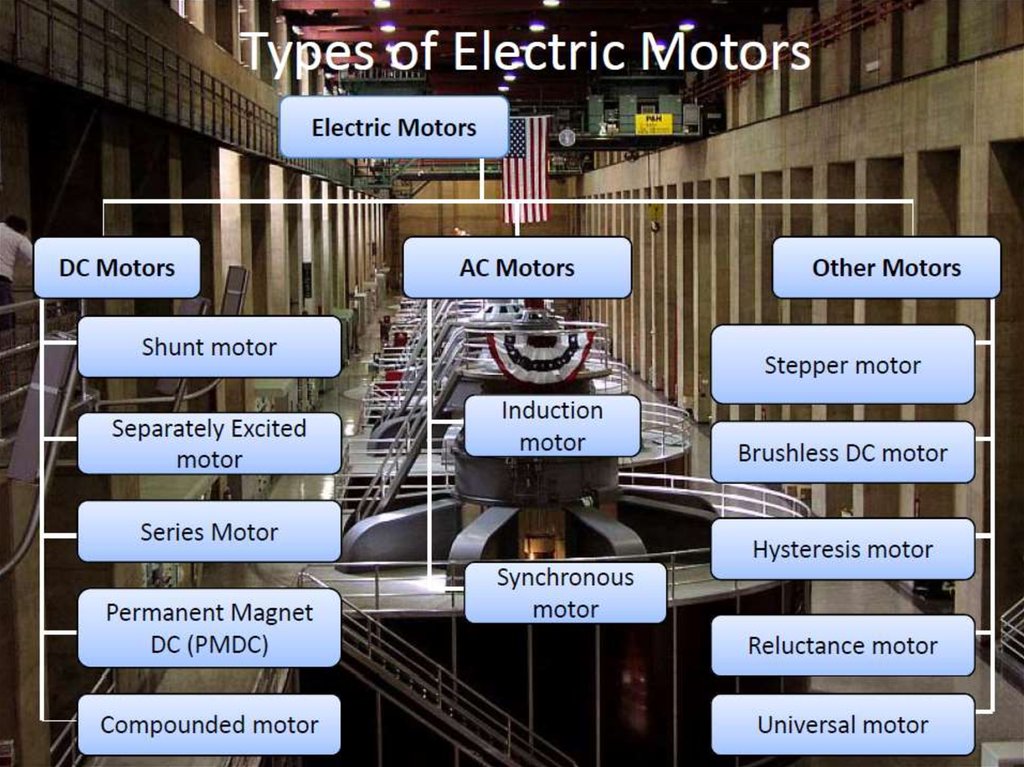
3. MOTOR CLASSIFICATION
An electric motor is a device which converts electrical energyinto kinetic energy (i.e. motion). Most motors described in this guide
[gaɪd] spin on an axis, but there are also specialty motors that move
linearly. All motors are either alternating current (AC) or direct current
(DC), but a few can operate on both. The following lists the most
common motors in use today. Each motor type has unique [juːˈniːk]
characteristics that make it suitable to particular applications.
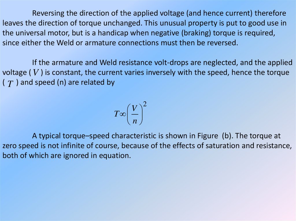
4.
5.
The direct current motor or the DC motor has a lot of applicationin today’s field of engineering and technology. Starting from an electric
shaver to parts of automobiles, in all small or medium sized motoring
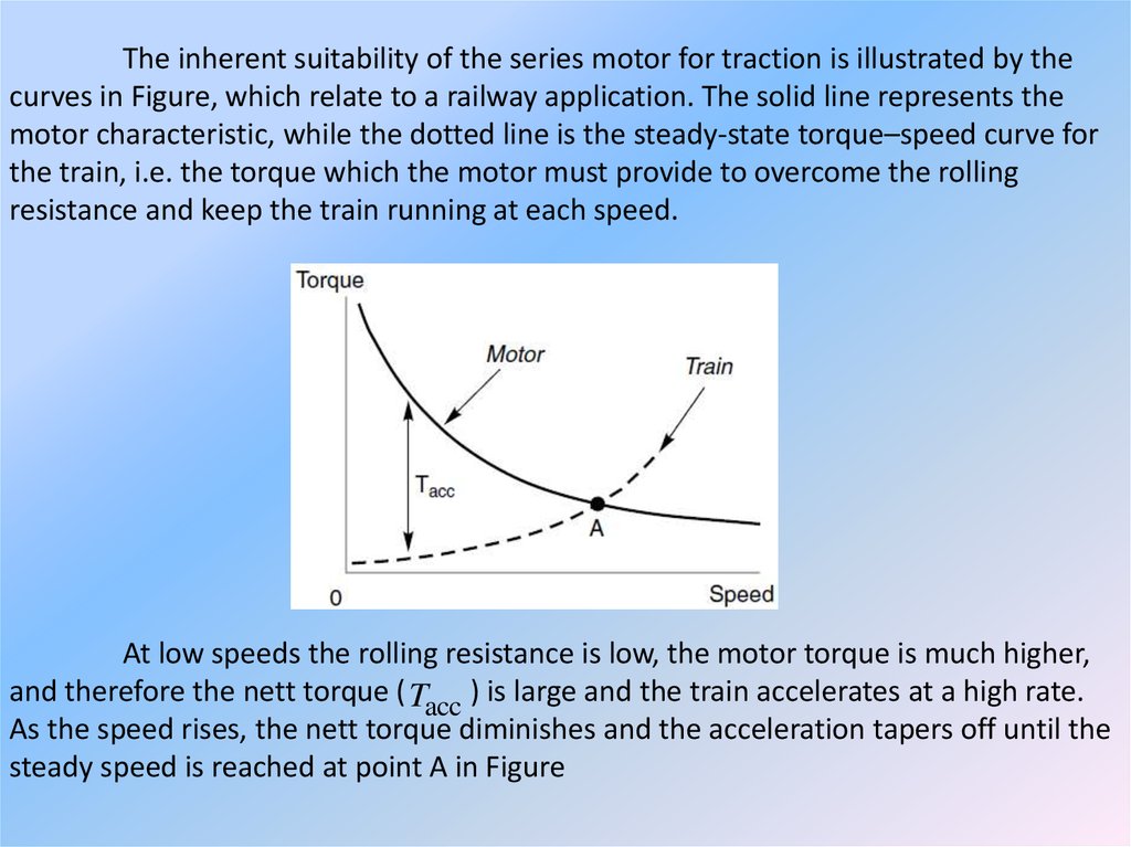
applications DC motors come handy. And because of its wide range of
application different functional types of DC motor are available in the
market for specific requirements.
The types of DC motor can be listed as follows-DC motor:
- Permanent Magnet DC Motor
- Separately Excited DC Motor
- Self Excited DC Motor
- Shunt Wound DC Motor
- Series Wound DC Motor
- Compound Wound DC Motor
- Short shunt DC Motor
- Long shunt DC Motor
- Differential Compound DC Motor
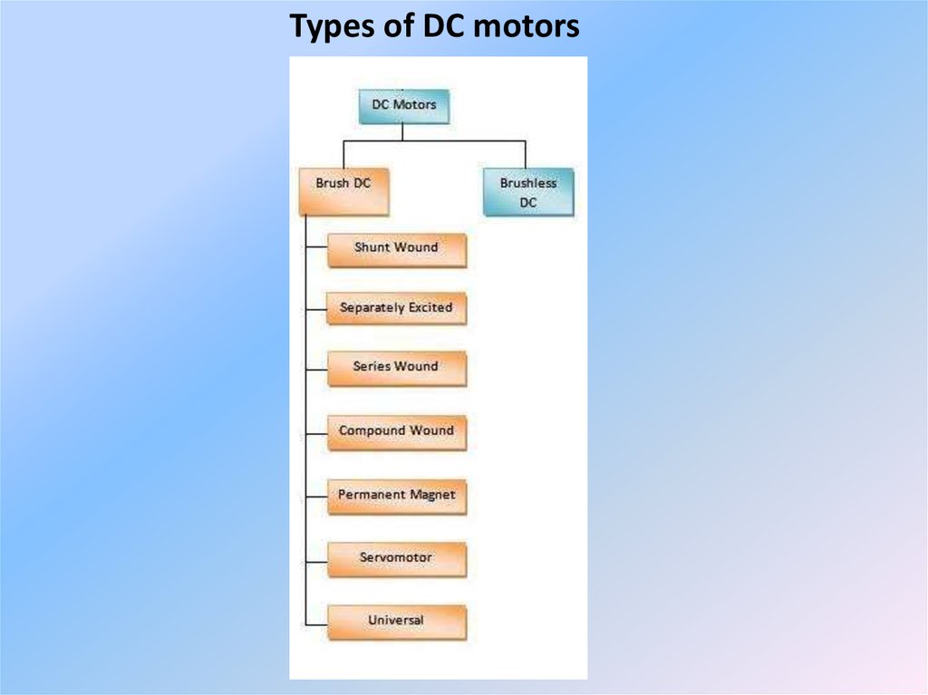
6.
Types of DC motors7.
DC motors are often used in applications where precise speedcontrol is required. They are divided into three sub-categories:
• series
• shunt
• compound
Advanced motors have been developed in recent years, a
number of which do not neatly fall within traditional motor
classifications. They are typically used in OEM applications.
Examples include:
• electronically commutated motors
• switched reluctance
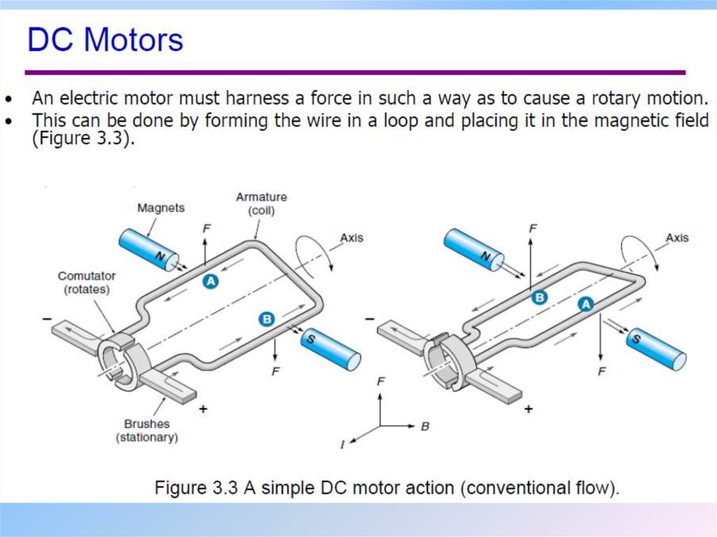
8. OPERATING PRINCIPLES
a) Major PartsAll motors have two basic parts:
• The STATOR (stationary part)
• The ROTOR (rotating part)
The design and fabrication of these two components determines
the classification and characteristics of the motor. Additional
components (e.g. brushes, slip rings, bearings, fans, capacitors,
centrifugal switches, etc.) may also be unique to a particular type of
motor.
b) Operation
The motors described in this guide all operate on the principle of
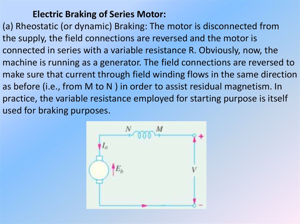
electromagnetism. Other motors do exist that operate on electrostatic
and Piezoelectric principles, but they are less common.
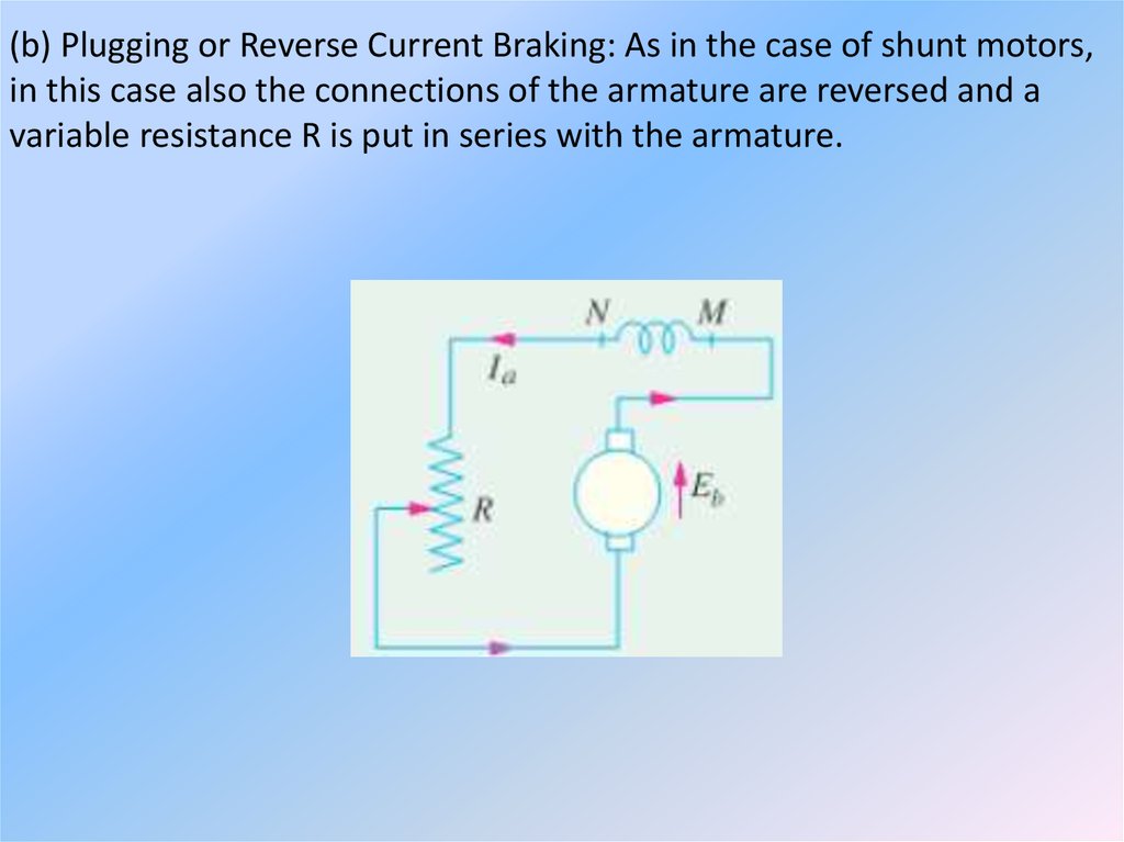
9.
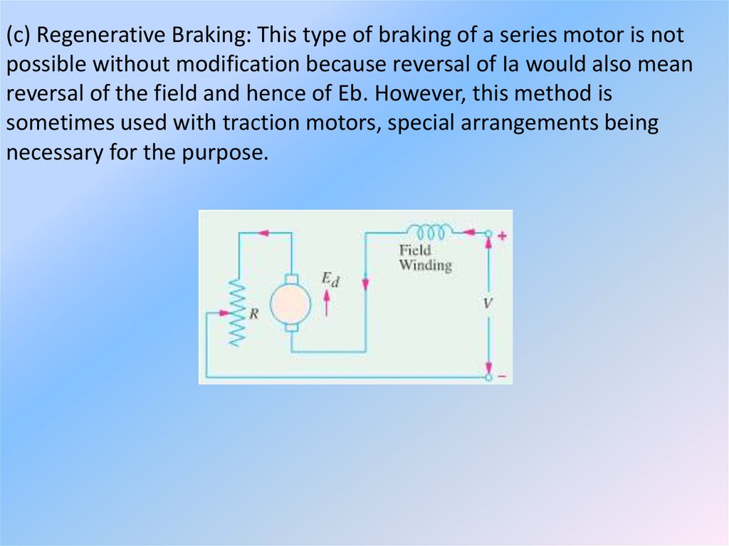
10.
11.
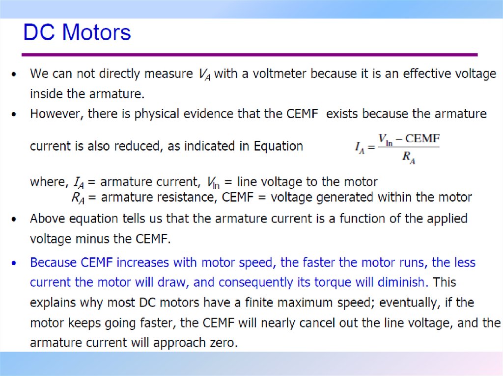
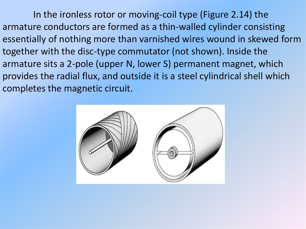
12. Motor’s Electrical Equations
The elevator is driven by a permanent-magnet DC motor. Theequivalent circuit of the permanent-magnet DC motor is confined to the
armature circuit which is illustrated in Figure
13.
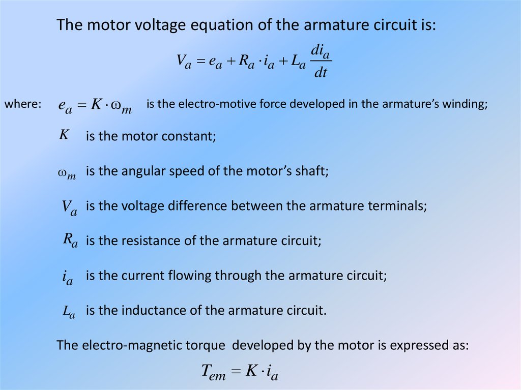
The motor voltage equation of the armature circuit is:Va ea Ra ia La
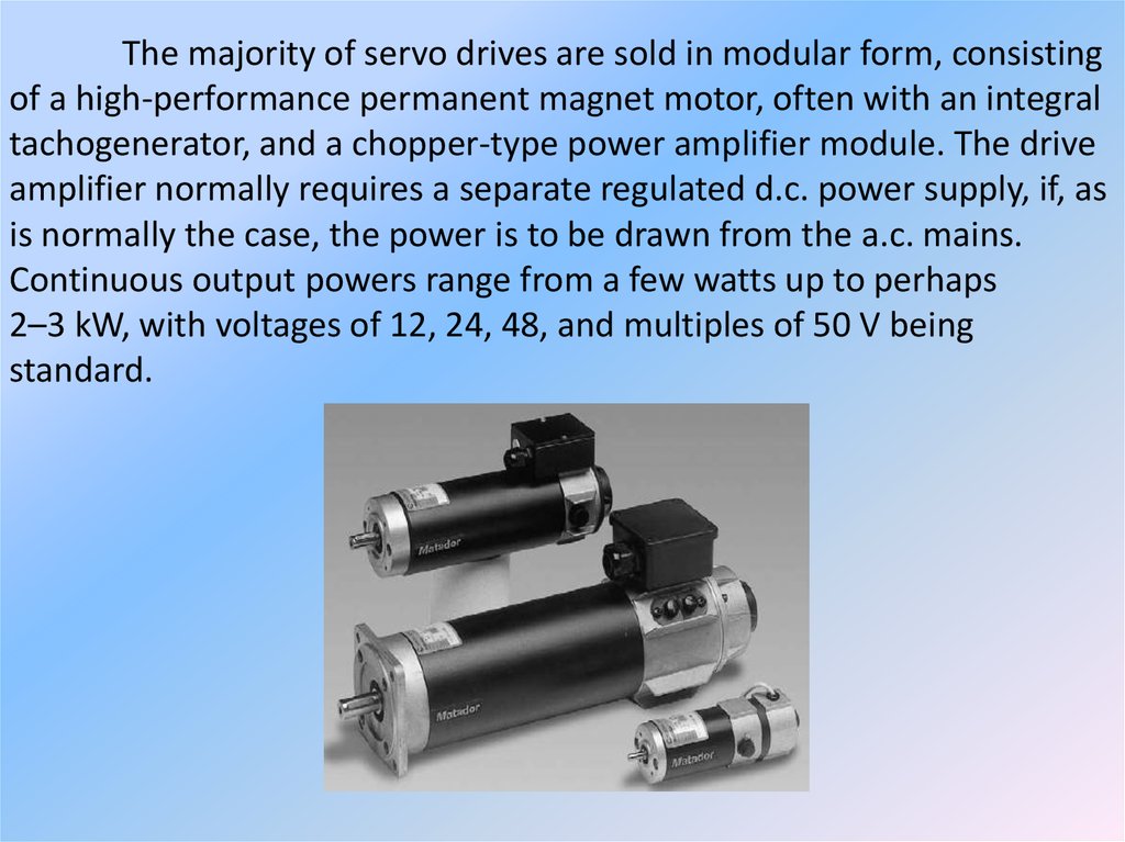
where:
dia
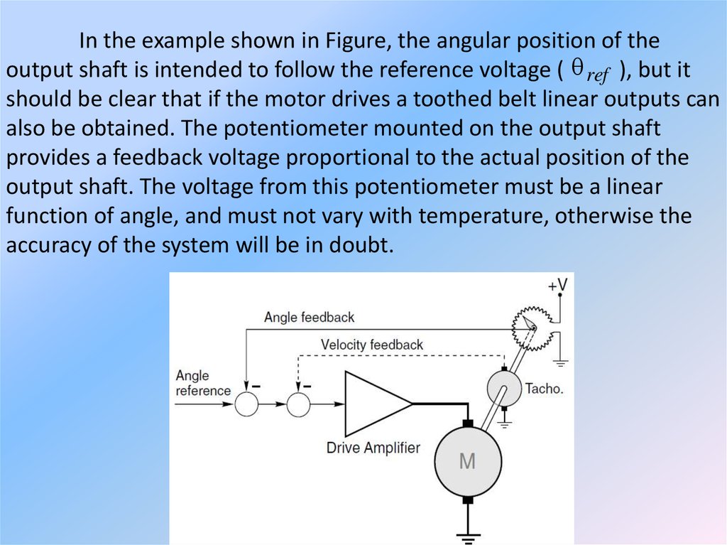
dt
ea K m is the electro-motive force developed in the armature’s winding;
K
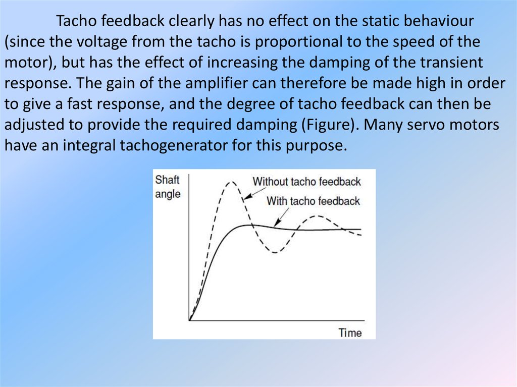
is the motor constant;
m is the angular speed of the motor’s shaft;
Va is the voltage difference between the armature terminals;
Ra is the resistance of the armature circuit;
ia is the current flowing through the armature circuit;
La is the inductance of the armature circuit.
The electro-magnetic torque developed by the motor is expressed as:
Tem K ia
14. Mechanical System’s Motion Equations
The motion equation of the entire system from the motor’s perspective is:d m
Tem J m
B m TL
dt
where: J m is the motor’s moment of inertia;
m is the angular speed of the rotor;
B
is the friction coefficient of the motor;
TL is the load torque placed on the motor’s shaft.
15.
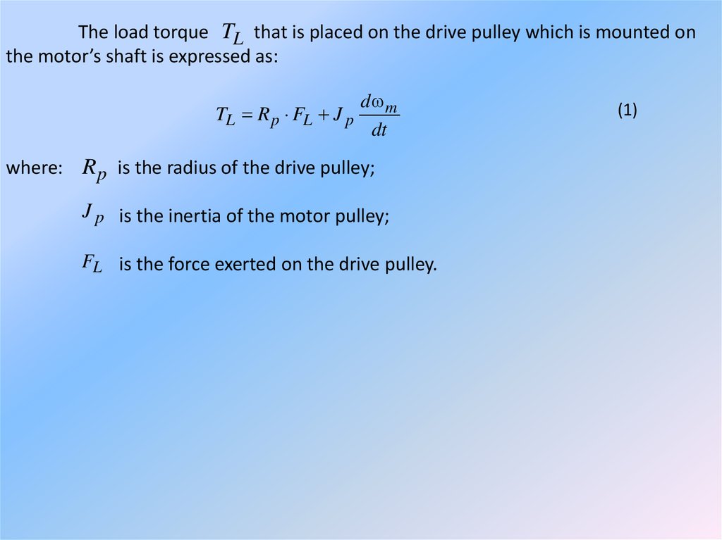
The load torque TL that is placed on the drive pulley which is mounted onthe motor’s shaft is expressed as:
TL R p FL J p
d m
dt
where: R p is the radius of the drive pulley;
J p is the inertia of the motor pulley;
FL is the force exerted on the drive pulley.
(1)
16.
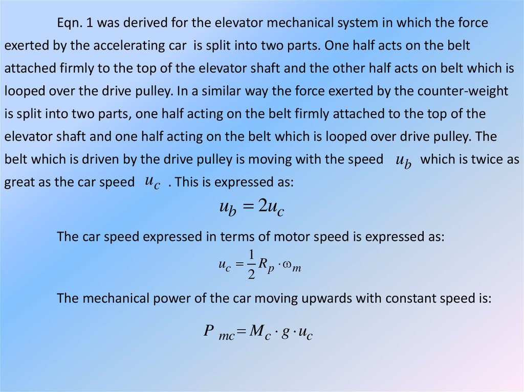
Eqn. 1 was derived for the elevator mechanical system in which the forceexerted by the accelerating car is split into two parts. One half acts on the belt
attached firmly to the top of the elevator shaft and the other half acts on belt which is
looped over the drive pulley. In a similar way the force exerted by the counter-weight
is split into two parts, one half acting on the belt firmly attached to the top of the
elevator shaft and one half acting on the belt which is looped over drive pulley. The
belt which is driven by the drive pulley is moving with the speed ub which is twice as
great as the car speed uc . This is expressed as:
ub 2uc
The car speed expressed in terms of motor speed is expressed as:
1
uc R p m
2
The mechanical power of the car moving upwards with constant speed is:
P mc M c g uc
17.
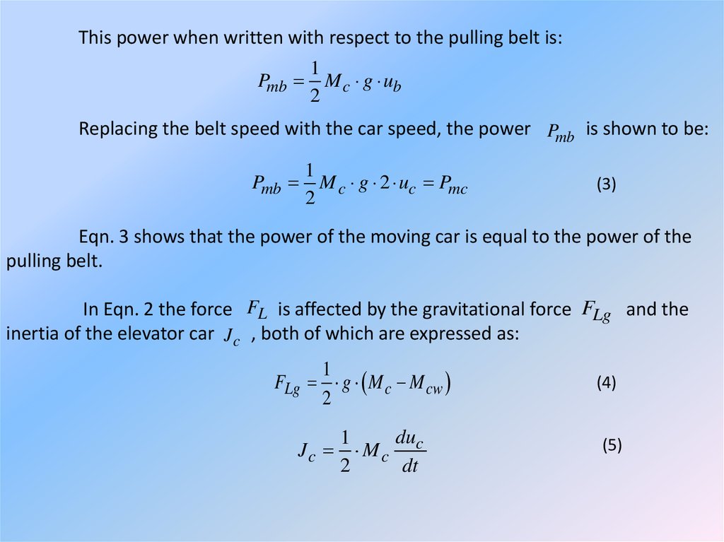
This power when written with respect to the pulling belt is:1
Pmb M c g ub
2
Replacing the belt speed with the car speed, the power Pmb is shown to be:
Pmb
1
M c g 2 uc Pmc
2
(3)
Eqn. 3 shows that the power of the moving car is equal to the power of the
pulling belt.
In Eqn. 2 the force FL is affected by the gravitational force FLg and the
inertia of the elevator car J c , both of which are expressed as:
1
FLg g M c M cw
2
Jc
du
1
Mc c
2
dt
(4)
(5)
18.
Eqn. 4 and Eqn. 5 hold only when the car is moving upwards and the belt isflexible; under these conditions the motor is not affected by the counter-weight during
acceleration. With this assumption Eqn. 1 can be inserted into Eqn. 2. The load torque
TL is now expressed as:
TL
d m
d m
1
1
R p g M c M cw R 2p M c
Jp
2
4
dt
dt
(6)
As mentioned, Eqn. 6 was derived for the elevator car moving upwards. When
the elevator car accelerates moving downwards the counter-weight’s mass M cw
should be considered while the elevator car’s mass M c should be ignored. The
equation for load torque TL when the elevator car is moving downwards has the
form:
d m
d m
1
1 2
TL R p g M cw M c R p M cw
Jp
2
4
dt
dt
19.
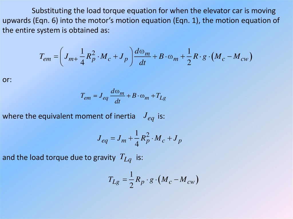
Substituting the load torque equation for when the elevator car is movingupwards (Eqn. 6) into the motor’s motion equation (Eqn. 1), the motion equation of
the entire system is obtained as:
1
1
d
Tem J m R 2p M c J p m B m R g M c M cw
4
2
dt
or:
Tem J eq
d m
B m TLg
dt
where the equivalent moment of inertia J eq is:
J eq J m
1 2
Rp M c J p
4
and the load torque due to gravity TLq is:
TLg
1
R p g M c M cw
2
20.
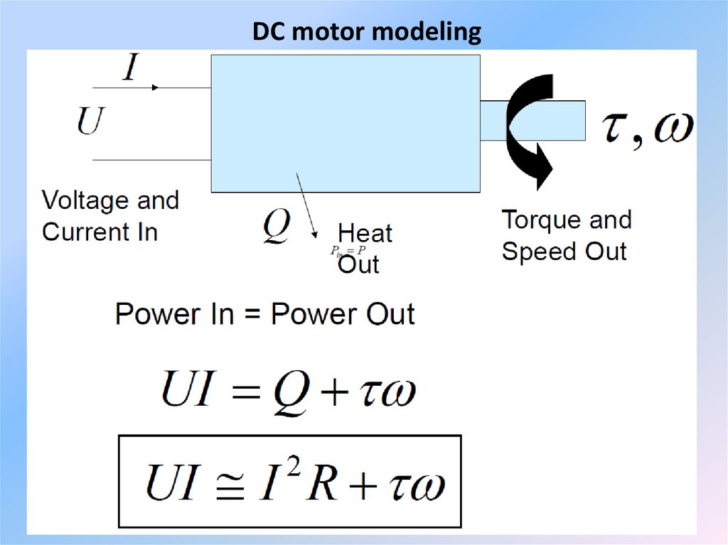
DC motor modeling21. DC motors
DC motors possess characteristics that make them attractive for certainapplications. For example, very high torque at low speeds makes the series DC motor
attractive for traction and engine starting applications.
Rotational speed can easily be controlled by varying the supply voltage.
The rotating part (rotor) of a DC motor is called the armature, and consists of
windings similar to those in a wound rotor induction motor
The stationary part (stator) introduces a magnetic field by either permanent
magnets or field windings which act on the armature.
22.
Current flows through the armature windings via carbon brushesand a commutator assembly. The commutator assembly is easily
recognizable as a ring of parallel diametrically opposite pairs of
rectangular shaped copper contacts at one end of the armature. Each
pair of contacts is connected to a coil wound on the armature. The
carbon brushes maintain contact with the commutator assembly via
springs. When the motor is turned on, current flows in through one
brush via a commutator contact connected to a coil winding on the
armature, and flows out the other carbon brush via a diametrically
opposite commutator contact.
23.
This causes the armature to appear as a magnet with which thestator field interacts. The armature field will attempt to align itself with
the stator field. When this occurs, torque is produced and the armature
will move slightly. At this time, connection with the first pair of
commutator contacts is broken and the next pair lines up with the
carbon brushes. This process repeats and the motor continues to turn.
24. Series motor – steady-state operating characteristics
The series connection of armature and Weld windings meansthat the Weld Flux is directly proportional to the armature current, and
the torque is therefore proportional to the square of the current.
Series-connected DC motor and steady-state torque–speed
curve
25.
Reversing the direction of the applied voltage (and hence current) thereforeleaves the direction of torque unchanged. This unusual property is put to good use in
the universal motor, but is a handicap when negative (braking) torque is required,
since either the Weld or armature connections must then be reversed.
If the armature and Weld resistance volt-drops are neglected, and the applied
voltage ( V ) is constant, the current varies inversely with the speed, hence the torque
( T ) and speed (n) are related by
V
T
n
2
A typical torque–speed characteristic is shown in Figure (b). The torque at
zero speed is not infinite of course, because of the effects of saturation and resistance,
both of which are ignored in equation.
26.
It is important to note that under normal running conditions thevolt drop across the series Weld is only a small part of the applied
voltage, most of the voltage being across the armature, in opposition to
the back e.m.f. This is of course what we need to obtain an efficient
energy conversion.
Under starting conditions, however, the back e.m.f. is zero, and if
the full voltage was applied the current would be excessive, being
limited only by the armature and Weld resistances. Hence for all but
small motors a starting resistance is required to limit the current to a
safe value.
27.
Returning to Figure (b), we note that the series motor differsfrom most other motors in having no clearly defined no-load speed, i.e.
no speed (other than infinity) at which the torque produced by the
motor falls to zero. This means that when running light, the speed of the
motor depends on the windage and friction torques, equilibrium being
reached when the motor torque equals the total mechanical resisting
torque. In large motors, the windage and friction torque is often
relatively small, and the no-load speed is then too high for mechanical
safety. Large series motors should therefore never be run uncoupled
from their loads. As with shunt motors, the connections to either the
Weld or armature must be reversed in order to reverse the direction of
rotation.
28.
Large series motors have traditionally been used for traction.Often, books say this is because the series motor has a high starting
torque, which is necessary to provide acceleration to the vehicle from
rest. In fact any d.c. motor of the same frame size will give the same
starting torque, there being nothing special about the series motor in
this respect. The real reason for its widespread use is that under the
simplest possible supply arrangement (i.e. constant voltage) the overall
shape of the torque–speed curve fits well with what is needed in
traction applications. This was particularly important in the days when it
was simply not feasible to provide any control of the armature voltage.
29.
The inherent suitability of the series motor for traction is illustrated by thecurves in Figure, which relate to a railway application. The solid line represents the
motor characteristic, while the dotted line is the steady-state torque–speed curve for
the train, i.e. the torque which the motor must provide to overcome the rolling
resistance and keep the train running at each speed.
At low speeds the rolling resistance is low, the motor torque is much higher,
and therefore the nett torque ( Tacc ) is large and the train accelerates at a high rate.
As the speed rises, the nett torque diminishes and the acceleration tapers off until the
steady speed is reached at point A in Figure
30.
Some form of speed control is obviously necessary in the example above ifthe speed of the train is not to vary when it encounters a gradient, which will result in
the rolling resistance curve shifting up or down. There are basically three methods
which can be used to vary the torque–speed characteristics, and they can be
combined in various ways.
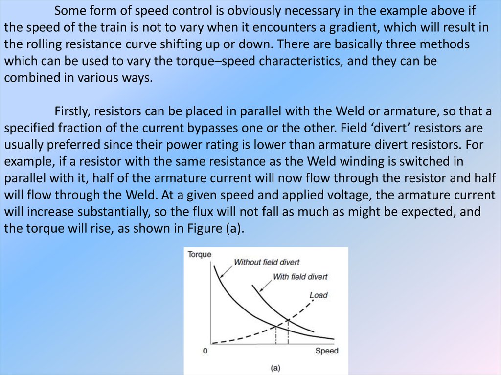
Firstly, resistors can be placed in parallel with the Weld or armature, so that a
specified fraction of the current bypasses one or the other. Field ‘divert’ resistors are
usually preferred since their power rating is lower than armature divert resistors. For
example, if a resistor with the same resistance as the Weld winding is switched in
parallel with it, half of the armature current will now flow through the resistor and half
will flow through the Weld. At a given speed and applied voltage, the armature current
will increase substantially, so the flux will not fall as much as might be expected, and
the torque will rise, as shown in Figure (a).
31.
This method is inefficient because power is wasted in the resistors, but issimple and cheap to implement. A more efficient method is to provide ‘tappings’ on
the Weld winding, which allow the number of turns to be varied, but of course this can
only be done if the motor has the tappings brought out.
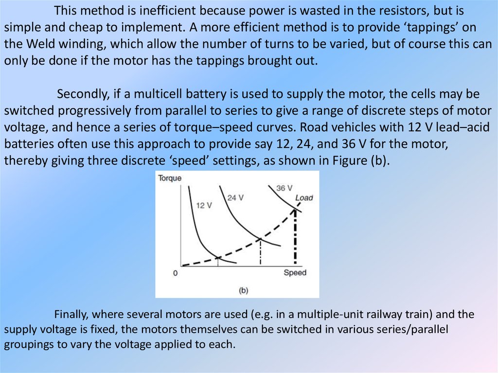
Secondly, if a multicell battery is used to supply the motor, the cells may be
switched progressively from parallel to series to give a range of discrete steps of motor
voltage, and hence a series of torque–speed curves. Road vehicles with 12 V lead–acid
batteries often use this approach to provide say 12, 24, and 36 V for the motor,
thereby giving three discrete ‘speed’ settings, as shown in Figure (b).
Finally, where several motors are used (e.g. in a multiple-unit railway train) and the
supply voltage is fixed, the motors themselves can be switched in various series/parallel
groupings to vary the voltage applied to each.
32.
Four-quadrant operation and regenerativebraking
The beauty of the separately excited d.c. motor is the ease with
which it can be controlled. Firstly, the steady-state speed is determined
by the applied voltage, so we can make the motor run at any desired
speed in either direction simply by applying the appropriate magnitude
and polarity of the armature voltage. Secondly, the torque is directly
proportional to the armature current, which in turn depends on the
difference between the applied voltage V and the back e.m.f. E. We can
therefore make the machine develop positive (motoring) or negative
(generating) torque simply by controlling the extent to which the
applied voltage is greater or less than the back e.m.f.
33.
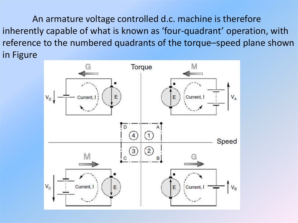
An armature voltage controlled d.c. machine is thereforeinherently capable of what is known as ‘four-quadrant’ operation, with
reference to the numbered quadrants of the torque–speed plane shown
in Figure
34.
Secondly, the supply voltage is shown by the old-fashioned battery symbol, asuse of the more modern circle symbol for a voltage source would make it more
difficult to differentiate between the source and the circle representing the machine
armature. The relative magnitudes of applied voltage and motional e.m.f. are
emphasised by the use of two battery cells when V E and one when V E .
We have seen that in a d.c. machine speed is determined by applied voltage
and torque is determined by current. Hence on the right-hand side of the diagram the
supply voltage is positive (upwards), while on the left-hand side the supply voltage is
negative (downwards). And in the upper half of the diagram current is positive (into
the dot), while in the lower half it is negative (out of the dot). For the sake of
convenience, each of the four operating conditions (A, B, C, D) have the same
magnitude of speed and the same magnitude of torque: these translate to equal
magnitudes of motional e.m.f. and current for each condition.
35.
If, with the motor running at position A, we suddenly reduce the supplyvoltage to a value which is less than the back e.m.f., the current (and hence torque)
will reverse direction, shifting the operating point to B in Figure. There can be no
sudden change in speed, so the e.m.f. will remain the same. If the new voltage is
chosen so that E Vb Va E , the new current will have the same amplitude as at
position A, so the new (negative) torque will be the same as the original positive
torque, as shown in Figure. But now power is supplied from the machine to the supply,
i.e. the machine is acting as a generator, as shown by the shaded arrow.
We should be quite clear that all that was necessary to accomplish this
remarkable reversal of power X ow was a modest reduction of the voltage applied to
the machine. At position A, the applied voltage was E I R , while at position B it
is E I R . Since IR will be small compared with E , the change ( 2 I R ) is also
small.
36.
Needless to say the motor will not remain at point B if left to itsown devices. The combined effect of the load torque and the negative
machine torque will cause the speed to fall, so that the back e.m.f. again
falls below the applied voltage VB, the current and torque become
positive again, and the motor settles back into quadrant 1, at a lower
speed corresponding to the new (lower) supply voltage. During the
deceleration phase, kinetic energy from the motor and load inertias is
returned to the supply. This is therefore an example of regenerative
braking, and it occurs naturally every time we reduce the voltage in
order to lower the speed.
37.
If we want to operate continuously at position B, the machinewill have to be driven by a mechanical source. We have seen above that
the natural tendency of the machine is to run at a lower speed than that
corresponding to point B, so we must force it to run faster, and create an
e.m.f greater than Vb , if we wish it to generate continuously.
It should be obvious that similar arguments to those set out
above apply when the motor is running in reverse (i.e. V is negative).
Motoring then takes place in quadrant 3 (point C), with brief excursions
into quadrant 4 (point D, accompanied by regenerative braking),
whenever the voltage is reduced in order to lower the speed.
38.
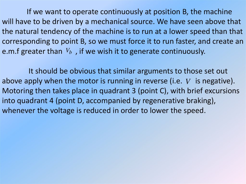
Separately Excited DC MotorThe field (or stator) coil contains a relatively large number of
turns which minimizes the current required to produce a strong stator
field (Figure). It is connected to a separate DC power supply, thus
making field current independent of load or armature current.
39.
Excellent speed regulation is characteristic of this design whichlends itself well to speed control by variation of the field current.
Separately excited DC motors can race to dangerously high
speeds (theoretically infinity) if current to the field coil is lost. Because of
this, applications should include some form of field current protection as
an unprotected motor could literally fly apart.
40. Compound DC Motor
The compound DC motor uses both series and shunt fieldwindings, which are usually connected so that their fields add
cumulatively (Figure).
This two winding connection
produces characteristics intermediate to
the shunt field and series field motors.
Speed regulation is better than
that of the series field motor.
41.
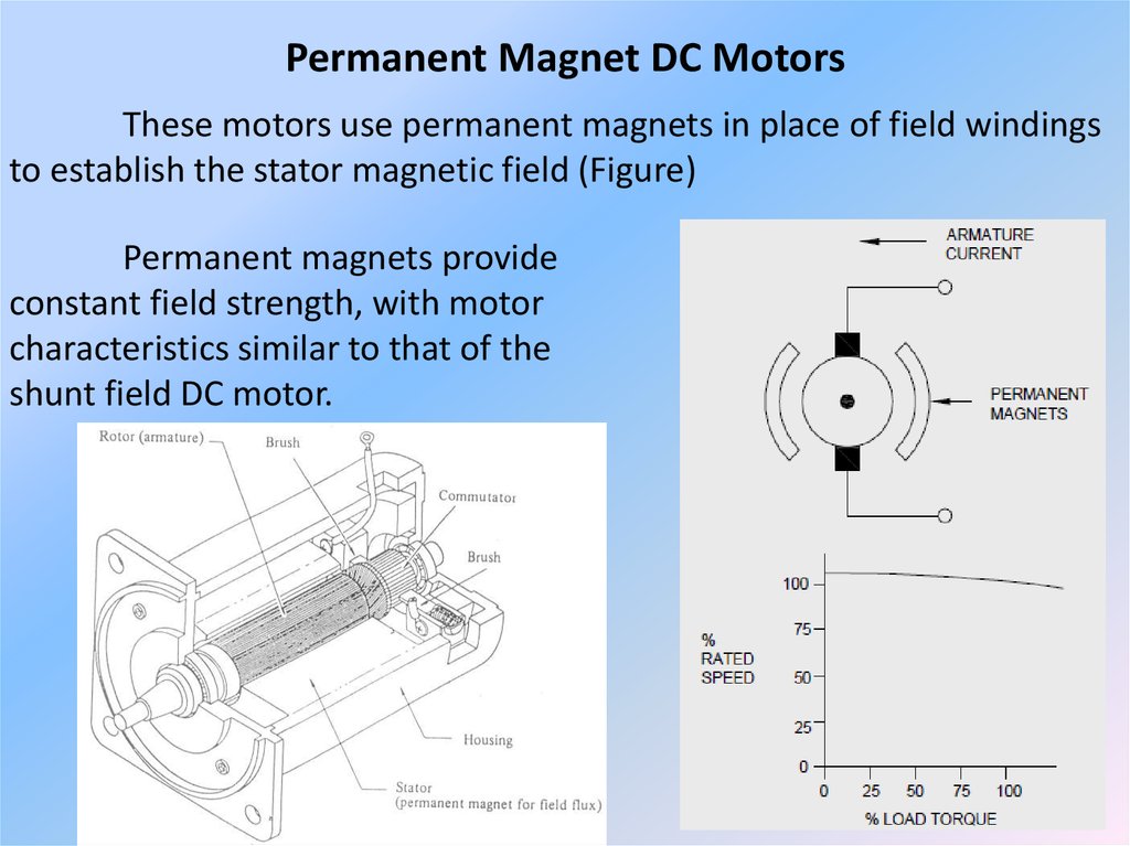
Permanent Magnet DC MotorsThese motors use permanent magnets in place of field windings
to establish the stator magnetic field (Figure)
Permanent magnets provide
constant field strength, with motor
characteristics similar to that of the
shunt field DC motor.
42.
Permanent magnet motors are often used in low horsepowerapplications, particularly those that are battery operated (e.g.
windshield wiper motor). However, with recent developments in magnet
technology, permanent magnet motors can be greater than 200 HP.
New high strength magnetic materials and power electronics
have been combined to produce high efficiency variable speed motors
ranging from sub fractional to multiple horse power units. Generally
these motors/controls are purpose built and are therefore incorporated
into OEM products.
43.
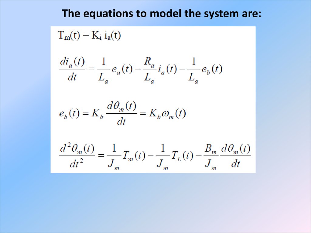
The equations to model the system are:44.
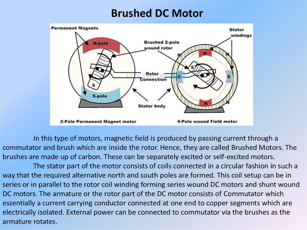
Brushed DC MotorIn this type of motors, magnetic field is produced by passing current through a
commutator and brush which are inside the rotor. Hence, they are called Brushed Motors. The
brushes are made up of carbon. These can be separately excited or self-excited motors.
The stator part of the motor consists of coils connected in a circular fashion in such a
way that the required alternative north and south poles are formed. This coil setup can be in
series or in parallel to the rotor coil winding forming series wound DC motors and shunt wound
DC motors. The armature or the rotor part of the DC motor consists of Commutator which
essentially a current carrying conductor connected at one end to copper segments which are
electrically isolated. External power can be connected to commutator via the brushes as the
armature rotates.
45. Electronically Commutated Motor (ECM)
An ECM is an electronically commutated permanent magnet DCmotor (Figure).
Electronics provide precisely
timed voltages to the coils, and use
rotation position sensors for timing.
The electronic controller can be
programmed to vary the torque speed
characteristics of the motor for a wide
variety of OEM applications such as fans
and drives.
46.
Although presently more costly than alternative motortechnologies, the higher efficiency and flexible operating characteristics
of these motors make them attractive.
An ECM is essentially a brushless DC motor with all speed.
Typical applications include variable torque drives for fans and pumps,
commercial refrigeration, and appliances.
For furnace fans, efficiency can be 20 to 30 percentage points
higher than a standard induction motor at full load. However, for
constant air circulation ECM’s have a definite advantage over standard
direct drive blower motors. At half speed, the ECM might consume as
little as 10% of the energy of a multi speed blower motor.
For appliances such as washing machines, the ECM can replace
the mechanical transmission due to wide range of torque speed
characteristics it can produce.
47. Thyristor d.c. drives – general
For motors up to a few kilowatts the armature converter can besupplied from either single-phase or three-phase mains, but for larger
motors three-phase is always used. A separate thyristor or diode
rectifier is used to supply the Weld of the motor: the power is much less
than the armature power, so the supply is often single-phase, as shown
in Figure
48.
The arrangement shown in Figure is typical of the majority of d.c.drives and provides for closed-loop speed control. The function of the
two control loops will be explored later, but readers who are not familiar
with the basics of feedback and closed-loop systems may find it helpful
to read through the Appendix at this point.
The main power circuit consists of a six-thyristor bridge circuit,
which rectifies the incoming a.c. supply to produce a d.c. supply to the
motor armature. The assembly of thyristors, mounted on a heatsink, is
usually referred to as the ‘stack’. By altering the Wring angle of the
thyristors the mean value of the rectified voltage can be varied, thereby
allowing the motor speed to be controlled.
49.
Low power control circuits are used to monitor the principalvariables of interest (usually motor current and speed), and to generate
appropriate Wring pulses so that the motor maintains constant speed
despite variations in the load. The ‘speed reference’ (Figure) is typically
an analogue voltage varying from 0 to 10 V, and obtained from a manual
speed-setting potentiometer or from elsewhere in the plant.
The combination of power, control, and protective circuits
constitutes the converter. Standard modular converters are available as
off-the-shelf items in sizes from 0.5 kW up to several hundred kW, while
larger drives will be tailored to individual requirements. Individual
converters may be mounted in enclosures with isolators, fuses etc., or
groups of converters may be mounted together to form a multi-motor
drive.
50. DC motor, a view inside
Simple, cheap.- Easy to control.
- 1W - 1kW
- Can be overloaded.
- Brushes wear.
- Limited overloading on
high speeds.
51.
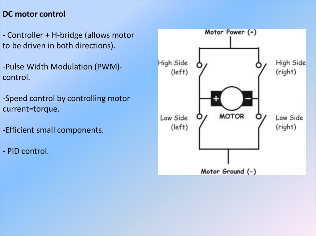
DC motor control- Controller + H-bridge (allows motor
to be driven in both directions).
-Pulse Width Modulation (PWM)control.
-Speed control by controlling motor
current=torque.
-Efficient small components.
- PID control.
52.
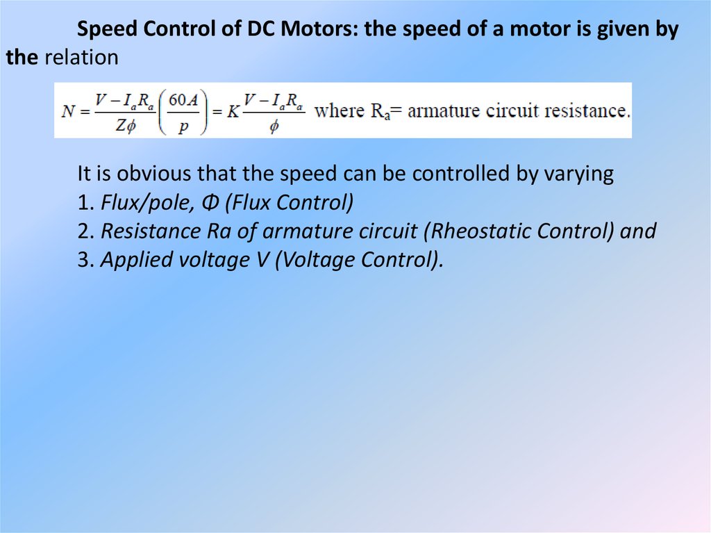
Speed Control of DC Motors: the speed of a motor is given bythe relation
It is obvious that the speed can be controlled by varying
1. Flux/pole, Φ (Flux Control)
2. Resistance Ra of armature circuit (Rheostatic Control) and
3. Applied voltage V (Voltage Control).
53.
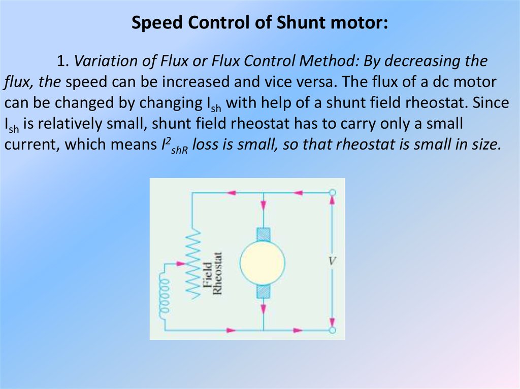
Speed Control of Shunt motor:1. Variation of Flux or Flux Control Method: By decreasing the
flux, the speed can be increased and vice versa. The flux of a dc motor
can be changed by changing Ish with help of a shunt field rheostat. Since
Ish is relatively small, shunt field rheostat has to carry only a small
current, which means I2shR loss is small, so that rheostat is small in size.
54.
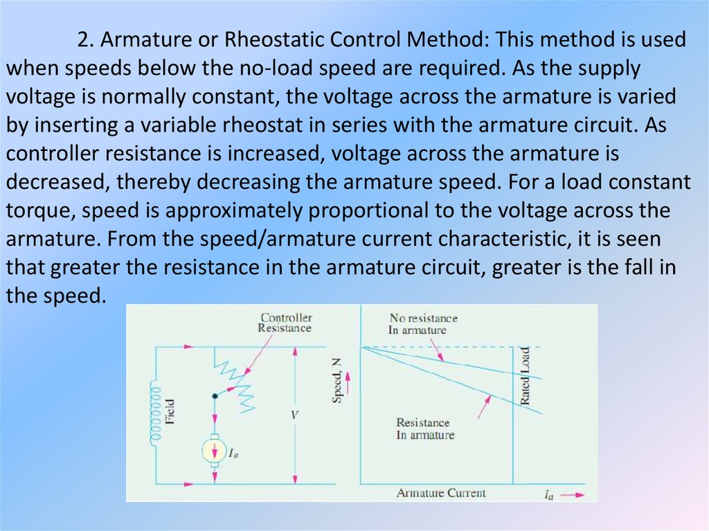
2. Armature or Rheostatic Control Method: This method is usedwhen speeds below the no-load speed are required. As the supply
voltage is normally constant, the voltage across the armature is varied
by inserting a variable rheostat in series with the armature circuit. As
controller resistance is increased, voltage across the armature is
decreased, thereby decreasing the armature speed. For a load constant
torque, speed is approximately proportional to the voltage across the
armature. From the speed/armature current characteristic, it is seen
that greater the resistance in the armature circuit, greater is the fall in
the speed.
55.
Voltage Control Method:(a) Multiple Voltage Control: In this method, the shunt field of
the motor is connected permanently to a fixed exciting voltage, but the
armature is supplied with different voltages by connecting it across one
of the several different voltages by means of suitable switchgear. The
armature speed will be approximately proportional to these different
voltages. The intermediate speeds can be obtained by adjusting the
shunt field regulator.
56.
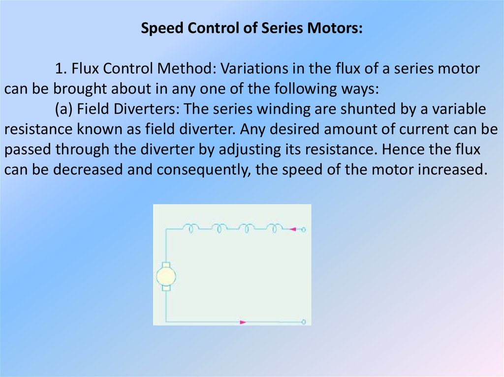
Speed Control of Series Motors:1. Flux Control Method: Variations in the flux of a series motor
can be brought about in any one of the following ways:
(a) Field Diverters: The series winding are shunted by a variable
resistance known as field diverter. Any desired amount of current can be
passed through the diverter by adjusting its resistance. Hence the flux
can be decreased and consequently, the speed of the motor increased.
57.
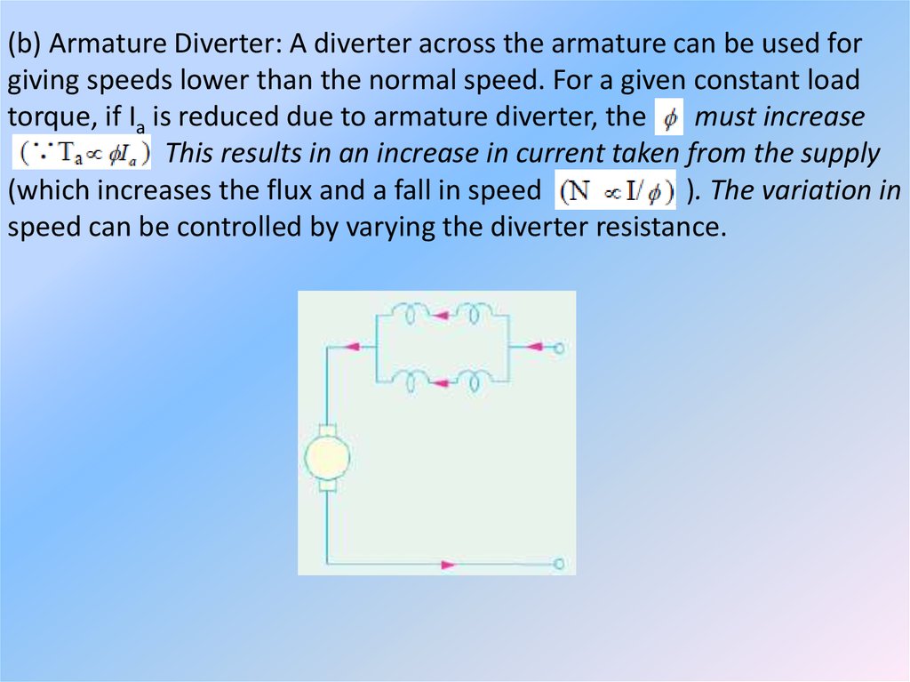
(b) Armature Diverter: A diverter across the armature can be used forgiving speeds lower than the normal speed. For a given constant load
torque, if Ia is reduced due to armature diverter, the
must increase
This results in an increase in current taken from the supply
(which increases the flux and a fall in speed
). The variation in
speed can be controlled by varying the diverter resistance.
58.
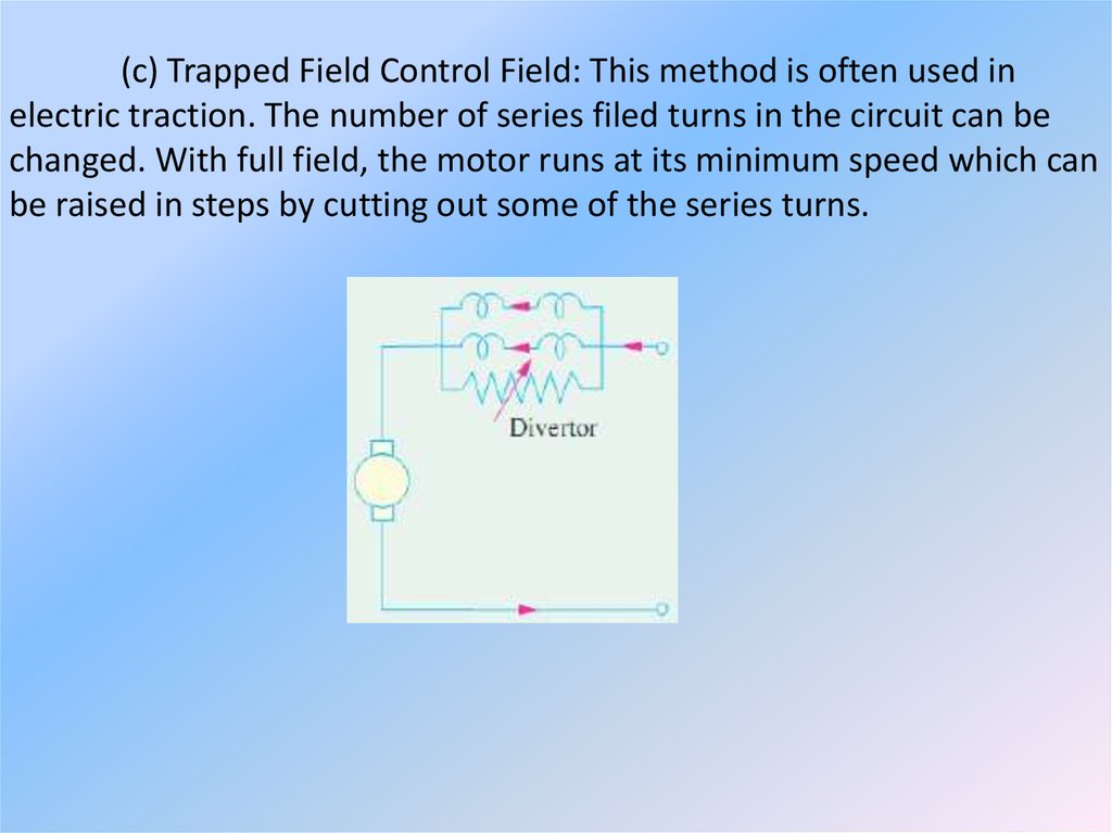
(c) Trapped Field Control Field: This method is often used inelectric traction. The number of series filed turns in the circuit can be
changed. With full field, the motor runs at its minimum speed which can
be raised in steps by cutting out some of the series turns.
59.
(d) Paralleling Field coils: this method used for fan motors,several speeds can be obtained by regrouping the field coils. It is seen
that for a 4-pole motor, three speeds can be obtained easily.
60.
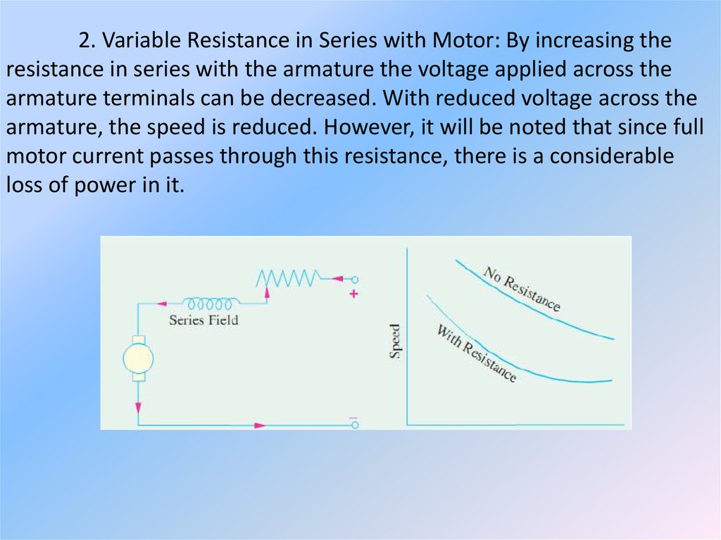
2. Variable Resistance in Series with Motor: By increasing theresistance in series with the armature the voltage applied across the
armature terminals can be decreased. With reduced voltage across the
armature, the speed is reduced. However, it will be noted that since full
motor current passes through this resistance, there is a considerable
loss of power in it.
61.
Electric Braking: A motor and its load may be brought to rest quicklyby using either (i) Friction Braking or (ii) Electric Braking. Mechanical
brake has one drawback: it is difficult to achieve a smooth stop because
it depends on the condition of the braking surface as well as on the skill
of the operator. The excellent electric braking methods are available
which eliminate the need of brake lining levers and other mechanical
gadgets. Electric braking, both for shunt and series motors, is of the
following three types:
(i) Rheostatic or dynamic braking
(ii) Plugging i.e., reversal of torque so that armature tends to
rotate in the opposite direction.
(iii) Regenerative braking.
Obviously, friction brake is necessary for holding the motor even after it
has been brought to rest.
62.
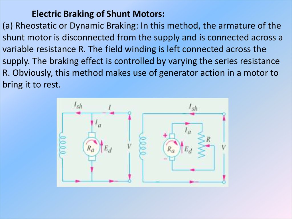
Electric Braking of Shunt Motors:(a) Rheostatic or Dynamic Braking: In this method, the armature of the
shunt motor is disconnected from the supply and is connected across a
variable resistance R. The field winding is left connected across the
supply. The braking effect is controlled by varying the series resistance
R. Obviously, this method makes use of generator action in a motor to
bring it to rest.
63.
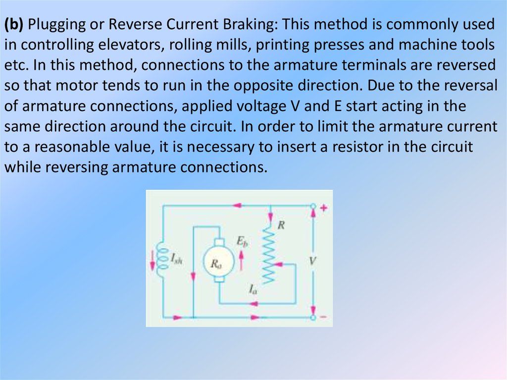
(b) Plugging or Reverse Current Braking: This method is commonly usedin controlling elevators, rolling mills, printing presses and machine tools
etc. In this method, connections to the armature terminals are reversed
so that motor tends to run in the opposite direction. Due to the reversal
of armature connections, applied voltage V and E start acting in the
same direction around the circuit. In order to limit the armature current
to a reasonable value, it is necessary to insert a resistor in the circuit
while reversing armature connections.
64.
(c) Regenerative Braking: This method is used when the load on themotor has over-hauling characteristic as in the lowering of the cage of a
hoist or the downgrade motion of an electric train.
Regeneration takes place when Eb becomes grater than V. This happens
when the overhauling load acts as a prime mover and so drives the
machines as a generator. Consequently, direction of Ia and hence of
armature torque is reversed and speed falls until E becomes lower than
V. It is obvious that during the slowing down of the motor, power is
returned to the line which may be used for supplying another train on
an upgrade, thereby relieving the powerhouse of part of its load.
65.
Electric Braking of Series Motor:(a) Rheostatic (or dynamic) Braking: The motor is disconnected from
the supply, the field connections are reversed and the motor is
connected in series with a variable resistance R. Obviously, now, the
machine is running as a generator. The field connections are reversed to
make sure that current through field winding flows in the same direction
as before (i.e., from M to N ) in order to assist residual magnetism. In
practice, the variable resistance employed for starting purpose is itself
used for braking purposes.
66.
(b) Plugging or Reverse Current Braking: As in the case of shunt motors,in this case also the connections of the armature are reversed and a
variable resistance R is put in series with the armature.
67.
(c) Regenerative Braking: This type of braking of a series motor is notpossible without modification because reversal of Ia would also mean
reversal of the field and hence of Eb. However, this method is
sometimes used with traction motors, special arrangements being
necessary for the purpose.
68. Servo motors
Although there is no sharp dividing line between servo motorsand ordinary motors, the servo type will be intended for use in
applications which require rapid acceleration and deceleration. The
design of the motor will reflect this by catering for intermittent currents
(and hence torques) of many times the continuously rated value.
Because most servo motors are small, their armature resistances are
relatively high: the short-circuit (locked-rotor) current at full armature
voltage is therefore perhaps only five times the continuously rated
current, and the drive amplifier will normally be selected so that it can
cope with this condition without difficulty, giving the motor a very rapid
acceleration from rest.
69.
The even more arduous condition in which the full armaturevoltage is suddenly reversed with the motor running at full speed is also
quite normal. (Both of these modes of operation would of course be
quite unthinkable with a large d.c. motor, because of the huge currents
which would flow as a result of the much lower per-unit armature
resistance.) Because the drive amplifier must have a high current
capability to provide for the high accelerations demanded, it is not
normally necessary to employ an inner current-loop of the type
discussed earlier.
In order to maximise acceleration, the rotor inertia must be
minimised, and one obvious way to achieve this is to construct a motor
in which only the electric circuit (conductors) on the rotor move, the
magnetic part (either iron or permanent magnet) remaining stationary.
This principle is adopted in ‘ironless rotor’ and ‘printed armature’
motors.
70.
In the ironless rotor or moving-coil type (Figure 2.14) thearmature conductors are formed as a thin-walled cylinder consisting
essentially of nothing more than varnished wires wound in skewed form
together with the disc-type commutator (not shown). Inside the
armature sits a 2-pole (upper N, lower S) permanent magnet, which
provides the radial flux, and outside it is a steel cylindrical shell which
completes the magnetic circuit.
71.
Needless to say the absence of slots to support the armaturewinding results in a relatively fragile structure, which is therefore limited
to diameters of not much over 1 cm. Because of their small size they are
often known as micromotors, and are very widely used in cameras,
video systems, card readers etc.
The printed armature type is altogether more robust, and is
made in sizes up to a few kilowatts. They are generally made in disc or
pancake form, with the direction of flux axial and the armature current
radial. The armature conductors resemble spokes on a wheel; the
conductors themselves being formed on a lightweight disc.
72.
Early versions were made by using printed-circuit techniques,but pressed fabrication is now more common. Since there are usually at
least 100 armature conductors, the torque remains almost constant as
the rotor turns, which allows them to produce very smooth rotation at
low speed. Inertia and armature inductance are low, giving a good
dynamic response, and the short and fat shape makes them suitable for
applications such as machine tools and disc drives where axial space is
at a premium.
73. DC servo drives
The precise meaning of the term ‘servo’ in the context of motorsand drives is difficult to pin down. Broadly speaking, if a drive
incorporates ‘servo’ in its description, the implication is that it is
intended specifically for closed-loop or feedback control, usually of shaft
torque, speed, or position. Early servomechanisms were developed
primarily for military applications, and it quickly became apparent that
standard d.c. motors were not always suited to precision control. In
particular high torque to inertia ratios were needed, together with
smooth ripple-free torque.
74.
Motors were therefore developed to meet these exactingrequirements, and not surprisingly they were, and still are, much more
expensive than their industrial counterparts. Whether the extra expense
of a servo motor can be justified depends on the specification, but
prospective users should always be on their guard to ensure they are
not pressed into an expensive purchase when a conventional industrial
drive could cope perfectly well.
75.
The majority of servo drives are sold in modular form, consistingof a high-performance permanent magnet motor, often with an integral
tachogenerator, and a chopper-type power amplifier module. The drive
amplifier normally requires a separate regulated d.c. power supply, if, as
is normally the case, the power is to be drawn from the a.c. mains.
Continuous output powers range from a few watts up to perhaps
2–3 kW, with voltages of 12, 24, 48, and multiples of 50 V being
standard.
76. Position control
As mentioned earlier many servo motors are used in closed-loopposition control applications, so it is appropriate to look briefly at how
this is achieved.
77.
In the example shown in Figure, the angular position of theoutput shaft is intended to follow the reference voltage ( ref ), but it
should be clear that if the motor drives a toothed belt linear outputs can
also be obtained. The potentiometer mounted on the output shaft
provides a feedback voltage proportional to the actual position of the
output shaft. The voltage from this potentiometer must be a linear
function of angle, and must not vary with temperature, otherwise the
accuracy of the system will be in doubt.
78.
The feedback voltage (representing the actual angle of the shaft)is subtracted from the reference voltage (representing the desired
position) and the resulting position error signal is amplified and used to
drive the motor so as to rotate the output shaft in the desired direction.
When the output shaft reaches the target position, the position error
becomes zero, no voltage is applied to the motor, and the output shaft
remains at rest. Any attempt to physically move the output shaft from
its target position immediately creates a position error and a restoring
torque is applied by the motor.
79.
The dynamic performance of the simple scheme describedabove is very unsatisfactory as it stands. In order to achieve a fast
response and to minimise position errors caused by static friction, the
gain of the amplifier needs to be high, but this in turn leads to a highly
oscillatory response which is usually unacceptable. For some fixed-load
applications, matters can be improved by adding a compensating
network at the input to the amplifier, but the best solution is to use
‘tacho’ (speed) feedback (shown dotted in Figure) in addition to the
main position feedback loop.
80.
Tacho feedback clearly has no effect on the static behaviour(since the voltage from the tacho is proportional to the speed of the
motor), but has the effect of increasing the damping of the transient
response. The gain of the amplifier can therefore be made high in order
to give a fast response, and the degree of tacho feedback can then be
adjusted to provide the required damping (Figure). Many servo motors
have an integral tachogenerator for this purpose.