946.85K

Категория:

Экономика

Macroeconomics. Lecture 5. Short-run macroeconomic dynamics: the selected models of business cycles

1.

Macroeconomics
Lecture 5.
Short-run macroeconomic dynamics: the selected
models of business cycles

What are business cycles? Perhaps, you know
something from the introductory level…
• The business cycles occur when economic activity speeds up
or slows down.
• The business cycles are swings in total national output,
income and employment, usually lasting for a period of 8 to
10 years, marked by widespread expansion or contraction in
many sectors of the economy.

3.

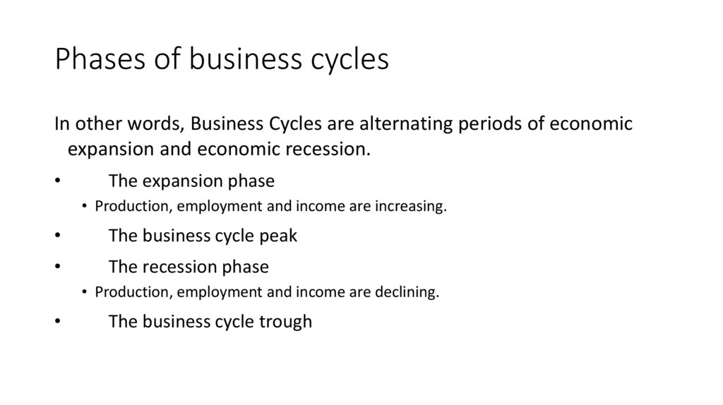
Phases of business cycles
In other words, Business Cycles are alternating periods of economic
expansion and economic recession.
The expansion phase
• Production, employment and income are increasing.
The business cycle peak
The recession phase
• Production, employment and income are declining.
The business cycle trough

4.

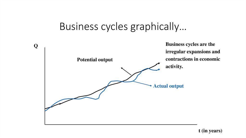
Business cycles graphically…
Q
Potential output
Business cycles are the
irregular expansions and
contractions in economic
activity.
Actual output
t (in years)

5.

Business cycles and unemployment dynamics
Recessions cause the unemployment rate to increase. We should
remember about frictional, structural and cyclical unemployment.
By the way, the rate of unemployment continues to be high after the
recession is over, because:
• Discouraged workers re-enter the labour force.
• Some workers have lost their skills.
• Firms continue to operate below capacity after the recession is
over and may not re-hire workers for some time.

6.

The most important recent recessions
1974/75: Oil price shock caused by OPEC.
1982/83: High real wages and inflation.
2008/09: World financial crisis – “The Great Recession”.
2020/21: Coronavirus pandemic – “The Great Lockdown”.

7.

How to explain business cycles?
?

8.

The multiplier-accelerator model as the
oldest formalized model of cycle
• Initial points
1.The model is a synthesis of the “Keynesian multiplier” and
the “accelerator” theory of investment
2.The accelerator model is based on the truism that, if
technology (and thus the capital/output ratio) is held
constant, an increase in output can only be achieved though
an increase in the capital stock.

9.

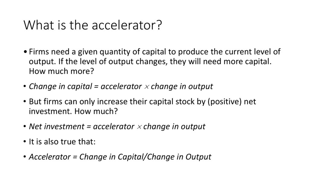
What is the accelerator?
• Firms need a given quantity of capital to produce the current level of
output. If the level of output changes, they will need more capital.
How much more?
• Change in capital = accelerator change in output
• But firms can only increase their capital stock by (positive) net
investment. How much?
• Net investment = accelerator change in output
• It is also true that:
• Accelerator = Change in Capital/Change in Output

10.

About constancy of the capital-output ratio
•If we do not allow for productivity boosting technical change,
then the capital output ratio is held constant.
•If fact, this is what we are assuming—no technical change.

11.

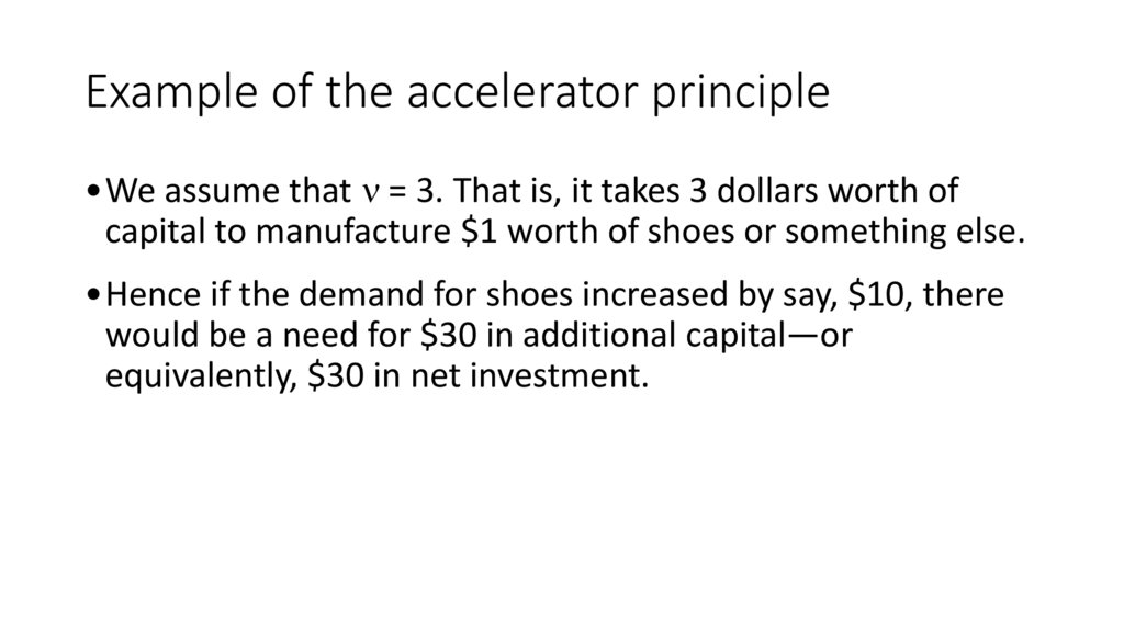
Example of the accelerator principle
•We assume that = 3. That is, it takes 3 dollars worth of
capital to manufacture $1 worth of shoes or something else.
•Hence if the demand for shoes increased by say, $10, there
would be a need for $30 in additional capital—or
equivalently, $30 in net investment.

12.

Formalizing the model (Part 1)
If the economy is in equilibrium,
then output supplied (Y) is equal to aggregate demand (AD).
Assuming a closed economy without government, we have:
Yt = Ct + It

13.

Formalizing the model (Part 2)
• The consumption function is given by:
Ct C cYt 1
• We assume that investment in the current period (It) is equal to some
fraction ( ) of change in output in the previous period (or lagged
output):
It (Yt 1 Yt 2)

14.

Combining these equations, we will receive:
Yt C (c v)Yt 1 Yt 2
• To simplify, we ignore the constant C
• To get a standardized form, let A = c + . Also, Let B = . Thus we can
write:
Yt At 1 Bt 2 0
• Note for the mathematically inclined: the last equation is a 2nd order
(homogenous) difference equation.

15.

Some essential ideas
• Change in investment affects output/income.
• Change in output/income affects (with delay) investment.
• Higher c and will lead to more unstable changes in the
macroeconomy.

16.

Some conclusions (derived from the
fundamental mathematical principles)
1.There will be cyclical fluctuations in the time path of national income
(Yt) if A2 < 4B.
2.If B = 1 (and presuming that A2 < 4B), then cycles are constant in
amplitude.
3.If B < 1 (and presuming that A2 < 4B), then cycles are damped—that
is, amplitude is a decreasing function of time.
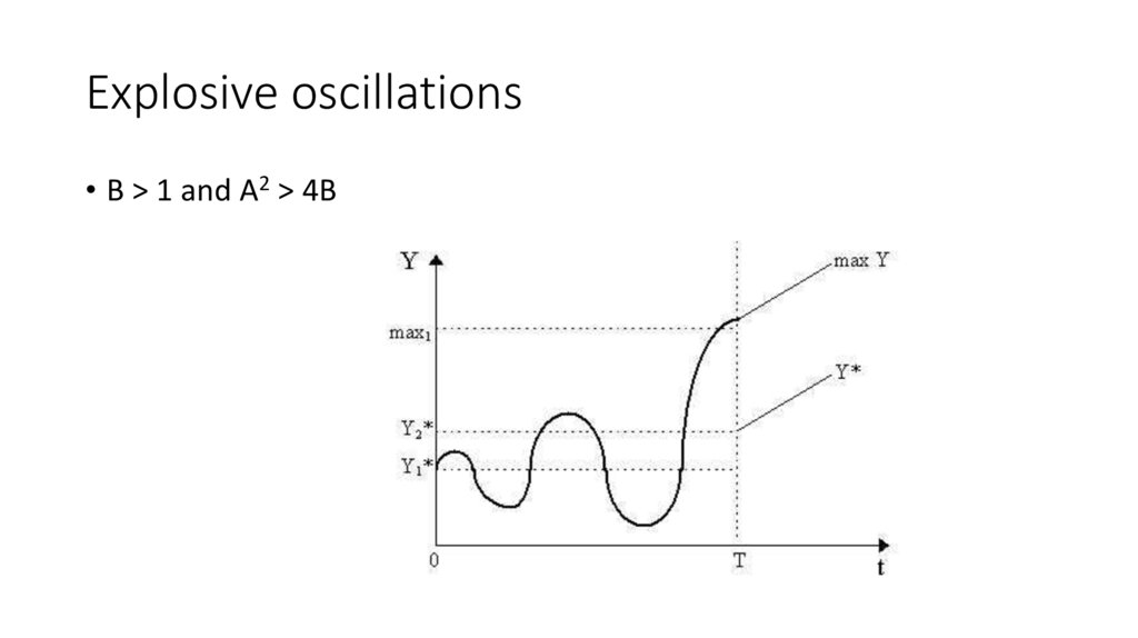
4.If B > 1 (and presuming that A2 < 4B), then cycles are explosive—that
is, amplitude is a increasing function of time.
5.There will be no cyclical fluctuations if A2 > 4B.

17.

Explosive oscillations
• B > 1 and A2 > 4B

18.

Limitations of the multiplier-accelerator
model
• This model is based on a crude theory of investment. There is no role for
“expected profits” or “animal spirits.” Furthermore, all relationships are linear.
There are no any determinants of investment except national income.
• The time lag between a change in output and a change in (net) investment can be
significant—the investment process (planning, finance, procurement,
manufacturing, installation, training) is often lengthy.
• For the economy as a whole, there is a limit to disinvestment (negative net
investment). At the aggregate level, the limit to capital reduction in a given period
is the wear and tear due to depreciation. Furthermore, there is a limit to increase
in output. The more sophisticated version of the model takes it into account.

19.

New Keynesian approach
• New Keynesian economists (Mankiw, Stiglitz, Akerlof and others)
believe that short-run fluctuations in output and employment
represent deviations from the “natural levels” (“potential GDP”, “full
employment”), and that these deviations occur because wages and
prices are sticky.
• If aggregate demand changes under the regime of the strickiness of
wages and prices, GDP and employment will fluctuate
• New Keynesian research attempts to explain the stickiness of wages
and prices by examining the microeconomics of price/wage
adjustment.

20.

Top reasons for sticky prices – Results from surveys of
managers (in the U.S.) (Mankiw, 2007)
- Coordination failure: firms hold back on price changes, waiting for others to go
first
- Firms delay raising prices until costs rise
- Firms prefer to vary other product attributes, such as quality, service, or delivery
lags
- Implicit contracts: firms tacitly agree to stabilize prices, perhaps out of ‘fairness’
to customers
- Explicit contracts that fix nominal prices (and wages)
- Menu costs

21.

The Real Business Cycle model
• All prices are flexible, even in short run:
• thus, money is “neutral” (that is, changes in money supply do not
affect real GDP and other real variables), even in short run.
• Fluctuations in output, employment, and other variables are the
optimal responses to exogenous changes in the economic
environment.
• Productivity shocks are the primary cause of economic fluctuations
(Kydland, 1982; Long, 1983; Prescott, 1989).

22.

Intertemporal substitution of labor
• In the RBC model, workers are willing to reallocate labor over
time in response to changes in the reward to working now
versus later.
• The intertemporal relative wage equals:
((1 + r)*w1)/w2
where w1 is the real wage rate in period 1 (the present) and
w2 is the real wage rate in period 2 (the future).

23.

The mechanism of cycles in the RBC model
• In the RBC model,
• productivity shocks cause fluctuations in the intertemporal relative
wage
• workers respond by adjusting labor supply
• this causes employment and output to fluctuate
• Critics argue that
• labor supply is not very sensitive to the intertemporal real wage
• high unemployment observed in recessions is mainly involuntary

24.

Are prices/wages flexible?
• The RBC model assumes that wages and prices are completely
flexible, so markets always clear.
• Proponents of the RBC model argue that the degree of
price stickiness occurring in the real world is not important for
understanding economic fluctuations. They also assume flexible
prices to be consistent with microeconomic theory.
• Critics believe that wage and price stickiness explains involuntary
unemployment (see above New Keynesian approach)

25.

The financial fragility hypothesis (aka the
financial instability hypothesis)
• Financial fragility hypothesis – developed by Hyman Minsky
(1919-1996) – states that over a period of good times, the
financial structures of a dynamic capitalist economy
endogenously evolve from being robust to being fragile, and
that once there is a “sufficient amount” of financially fragile
firms, the economy becomes susceptible to debt deflations
and crises.
• It is very important how firms-borrowers finance their
investment in fixed capital!

26.

The classification of borrowers (and regimes
of financing)
• Minsky identified three types of borrowers that contribute to the
accumulation of debt:
1) The "hedge borrower" can make debt payments (covering
interest and principal) from current cash flows from investments.
2) For the "speculative borrower", the cash flow from investments
can service the debt, i.e., cover the interest due, but the borrower
must regularly roll over, or re-borrow, the principal.
3) The "Ponzi borrower" borrows based on the belief that the
appreciation of the value of the asset will be sufficient to refinance
the debt but could not make sufficient payments on interest or
principal with the cash flow from investments.

27.

Reasons for the name “Ponzi finance” or
“Ponzi regime”
• Named after Charles Ponzi (1882-1949), an Italian citizen
who launched the following scheme during 1918-1920 in the
USA: “pay early investors returns from the investments of
later investors.”
• He was sentenced in 1920 and spent 12 years in jail. Died in
Rio da Janeiro.

28.

The theory of firm’s investment decision
graphically

29.

Some explanations
• I is investment
• PK is the demand price of investment (willingness to pay some
amount of money for capital equipment by the firm); it is adjusted for
the borrower’s risk (fear to not to repay debt)
• PI is the supply price of investment (actual price of capital equipment
for the firm); it is adjusted for the lender’s risk (fear of not to receive
back money lent)
• Investment will take place if the demand price exceeds the supply
price

30.

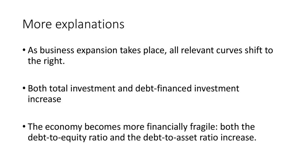
More explanations
• As business expansion takes place, all relevant curves shift to
the right.
• Both total investment and debt-financed investment
increase
• The economy becomes more financially fragile: both the
debt-to-equity ratio and the debt-to-asset ratio increase.

31.

The business expansion based on the
accumulation of financial fragility graphically

32.

The stages of business cycles according to the
financial fragility hypothesis
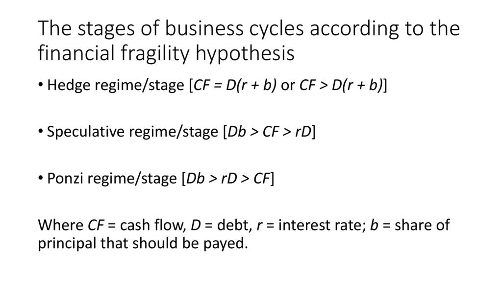
• Hedge regime/stage [CF = D(r + b) or CF > D(r + b)]
• Speculative regime/stage [Db > CF > rD]
• Ponzi regime/stage [Db > rD > CF]
Where CF = cash flow, D = debt, r = interest rate; b = share of
principal that should be payed.

33.

The hedge phase
• Conservative estimates of cash flows when making financial
decisions; business plans provide more than enough cash
generation to pay off cash commitments.
• Debt tends to be conservative and at long term fixed interest
rates
• This is a phase dominated by borrowers, (mostly companies)
who can fulfill their debt payments (interests and principals)
to creditors (mostly banks) from their cash flows.

34.

The speculative phase
• Estimates of cash flows are more aggressive - expected cash
inflows provide just enough to cover to make interest
payments on debts with principal rolled over.
• Debt becomes shorter term and therefore needs regular
refinancing; borrowers become exposed to short term
changes in lender’s willingness to extend loans
• The 'speculative phase' is dominated by borrowers,
(including governments and households) that are capable of
servicing their interests on their debts from their incoming
revenues.

35.

The “Ponzi” stage
• Estimates of cash generation not expected to cover cash
commitments.
• Debt is short term and rolled over
• The majority of borrowers in the system are unable to pay
even the interests on their debts (let alone the principals)
from their revenues.

36.

The Minsky moment and financial crisis
• If the use of Ponzi finance is general enough in the financial system,
then the inevitable disillusionment of the Ponzi borrower can cause
the system to seize up.
• When the speculative borrower can no longer refinance (roll over) the
principal even if able to cover interest payments, such agent can go
bankrupt too.
• Collapse of the speculative borrowers can then bring down even
hedge borrowers, who are unable to find loans despite the apparent
soundness of the underlying investments.
• At this stage, debt payments can only be settled by liquidating the
real assets of borrowers - the moment of deleveraging and default.
This situation is now called "Minsky's Moment"

37.

Some picture…

38.

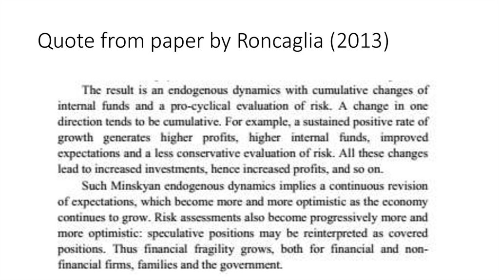
Quote from paper by Roncaglia (2013)

39.

Minsky about the policy
• Minsky observes that the government intervention (proper
fiscal policy measures) are necessary but not sufficient to
deal with such a financial crisis.
• They have to supplemented with strong regulatory and
superviory measures on the financial system.

40.

More about the “proper” fiscal policy
• Fiscal policy may have a discretionary component, such as the
introduction of new taxes in a boom or new spending in a downturn.
• However the discretionary action usually comes with a long lag, when
it comes at all: The goal was to present a structure of capitalism that
would be more prosperous and stable.
• Minsky stressed that "the budget structure must have the built-in
capacity" to produce sizable deficits when the economy plunges, and
to run surpluses during inflationary booms. (suggestion on automatic
stabilizers)

41.

The fiscal policy may not be enough
• Governments alone may not be enough to stabilize the
economy.
• In a recession, if a big firm or bank defaults on its debt, it can
also bring down others in the economy due to the
interlocking nature of their balance sheets. This could cause
a “snowball effect” on the economy.
• An additional constraining institution is needed to prevent
debt deflation from occurring.

42.

Paradox of tranquility
Government intervention is needed to stabilize the economy...
If policies are successful, the economy booms. Expectations
about the future returns become increasingly optimistic. As
mentioned before, riskier behavior is awarded.
This leads to fragility in the economy.

43.

What about the monetary policy?
• Monetary policy can constrain undue expansion and inflation
operates by way of disrupting financing markets and asset
values.
• Monetary policy to induce expansion operates by interest
rates and the availability of credit, which do not yield
increased investment if current and anticipated profits are
low.

44.

More about the monetary policy
• The Central Bank will generally be taking up the role of the
lender of last resort. The Central Bank will lend to financial
institutions. By lending to them, especially to the big
financial institutions, the Central Bank prevents big financial
institutions from defaulting.
• One problem with being the lender of last resort is that if
banks know that the central banks will always step in if the
borrower defaults, banks will have nothing to worry about.
Risky behavior is rewarded.
• There is, therefore, a need to supervise the private banks to
decrease the number of bad loans they approve.

45.

Results of the active government intervention
for the U.S. economy (Tymoigne, 2008)

46.

Stability is destabilizing!
• Profit-seeking firms have incentives to leverage and borrow
more against equity as long as the economy appears to be
stable.
• Therefore, “stability is destabilizing.” People take on more
and more risk.
• Capitalist economy based on fractional reserve banking
system is inherently unstable!

47.

Let me give examples of three empirical studies of the
financial fragility’s evolution in different countries
• Beshenov, S., and Rozmainsky, I. V. (2015). Hyman Minsky's Financial
Instability Hypothesis and the Greek Debt Crisis. Russian Journal of
Economics 1(4): 419–438.
• Nishi, H (2019). An empirical contribution to Minsky’s financial
fragility: Evidence from non-financial sectors in Japan. Cambridge
Journal of Economics 43(3): 585–622.
• Rozmainsky, I. V. and Selitsky, M. S. (2021). The financial instability
hypothesis and the case of private non-financial firms in South
Korea. AlterEconomics 18(3): 417–432. (In Russian).

48.

Empirical analysis of the Greek companies’ financing regimes
on the base of the financial fragility hypothesis from (Beshenov
and Rozmainsky, 2015)
• We used the financial statements for 36 companies from 2001 to
2014.
• The annual statements for Greek companies were taken from the
Bloomberg terminal.
• 36 companies were sampled based on the ASE General Index.
• ASE = the Athens Stock Exchange.

49.

Some details about this analysis and this
index
• The ASE General Index includes 60 of the largest Greek companies,
weighted in terms of capitalization.
• Why 36 instead of 60? Because selected companies satisfied with the
following criteria:
• The company belongs to the real sector
• We managed to find most of the information about the company for
the analysis (over 80%).
• The company had not been taken over by or merged with another
company during the period in question. Bankrupt companies were
also included in the sample.

50.

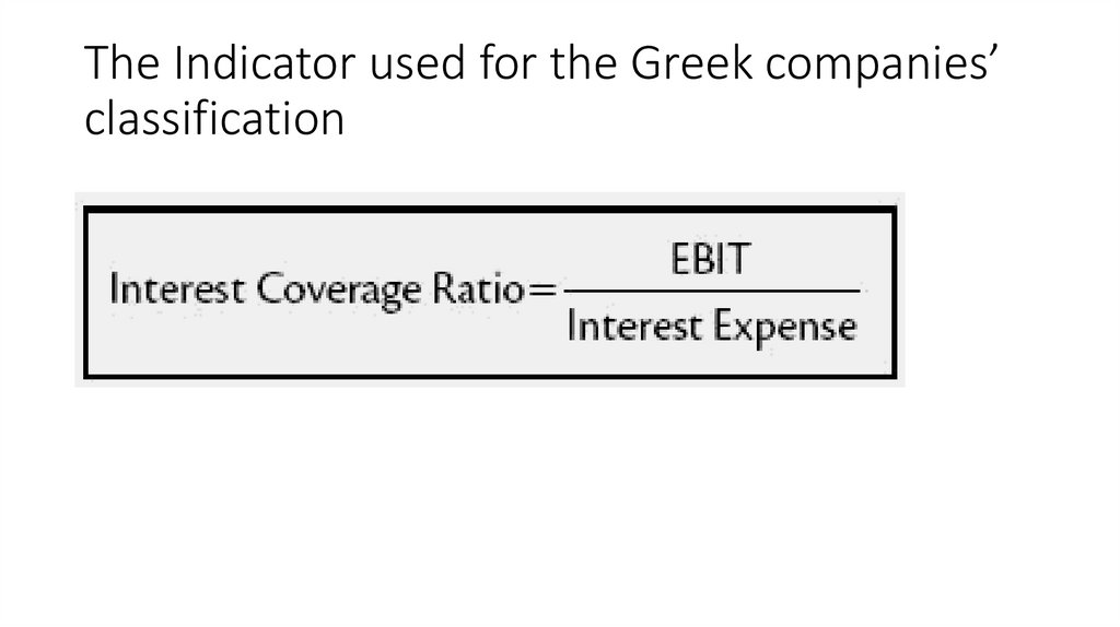
The Indicator used for the Greek companies’
classification

51.

Explanation of the Indicator
• EBIT = earnings before interest and taxes
• Interest Coverage Ratio (ICR) = interest payable on the company’s
borrowings
• ICR lets a financial statement analyst determine the company’s ability
to meet its obligations to repay loans.
• According to practical experts, a company that is financially stable and
robust, will have a ICR over 3 (Damodaran, 2011).

52.

The Principles of The Greek companies’
classification
• ICR>=3 treated as a financially “healthy” company or as a
company using Hedge Finance
• 3>=ICR>0 treated as a company exposed to financial shocks
and has a potential for fulfilling (incompletely) financial
obligations or as a company using Speculative Finance
• ICR=<0 treated as a company moving to bankruptcy and has no
potential for fulfilling financial obligations or as a company
using Ponzi Finance
• At the present moment there are more sophisticated
approaches to classify firms (see one example below)

53.

The dynamics of 36 Greek companies during
the period in question
• After 2001 the number of companies with speculative and Ponzi
finance increased.
• By the end of 2008, the share of companies with fragile financing rose
to 61% of the total number of analyzed companies (22 out of 36).
• By 2013, financially stable companies accounted for 17% of the
sample, which is the evidence of the deep recession.
• 3 companies were officially declared bankrupt.

54.

The essential diagram (2001-2014)

55.

Some Conclusions
• Experience of the Greek economy is consistent with the FIH.
• In the 2000s, the private business accumulated financial fragility
inside the Greek economy
• The crash of the Greek economy in 2015 can be treated as an effect of
accumulation of financial fragility

56.

Analysis of the financial fragility’s evolution in
Japan (Nishi, 2019)
• Nishi analyzed firms of different sizes and different sectors
• Nishi offered another index for measuring financial fragility on the
base of the next idea:

57.

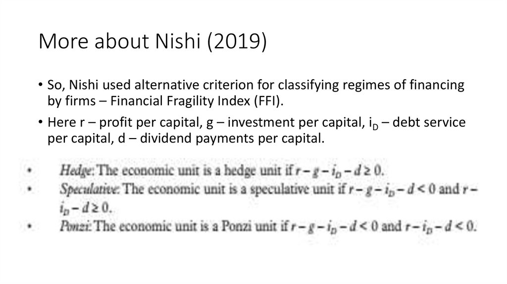
More about Nishi (2019)
• So, Nishi used alternative criterion for classifying regimes of financing
by firms – Financial Fragility Index (FFI).
• Here r – profit per capital, g – investment per capital, iD – debt service
per capital, d – dividend payments per capital.

58.

Evolution of financial fragility for Large
Manufacturing Japanese firms (1975-2015)

59.

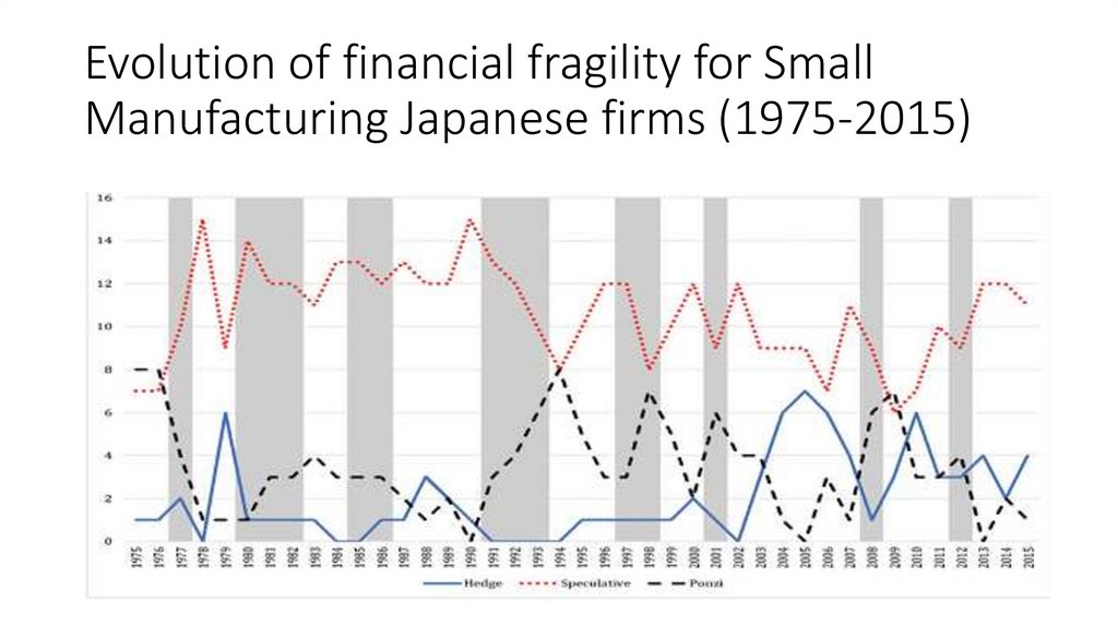
Evolution of financial fragility for Small
Manufacturing Japanese firms (1975-2015)

60.

Evolution of financial fragility for Large NonManufacturing Japanese firms (1975-2015)

61.

Evolution of financial fragility for Small NonManufacturing Japanese firms (1975-2015)

62.

Some conclusions from Nishi (2019)
1. Ponzi finance becomes popular before and during the recessions.
2. See this quotation

63.

The example of latest research – for the South Korean
private nonfinancial firms (Rozmainsky, Selitsky, 2021)
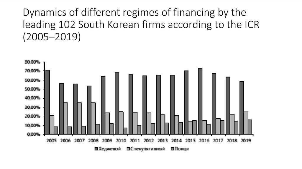
• The authors also analyzed firms of different sectors
• The authors used different criteria for estimating of the financial
fragility’s evolution.
• Some conclusions – see quotation: