The impact of credit supply shocks in the euro area: market-based financing versus loans

1.

Working Paper Series
Kristina Barauskaitė, Anh D. M. Nguyen,
Linda Rousová, Lorenzo Cappiello
The impact of credit supply shocks in
the euro area:
market-based financing versus loans
No 2673/ June 2022
Disclaimer: This paper should not be reported as representing the views of the European Central Bank
(ECB). The views expressed are those of the authors and do not necessarily reflect those of the ECB.

2.

Abstract
Using a novel quarterly dataset on debt financing of non-financial corporations, this paper
provides the first empirical evaluation of the relative importance of loan and market-based
finance (MBF) supply shocks on business cycles in the euro area as a whole and in its five
largest countries. In a Bayesian VAR framework, the two credit supply shocks are identified
via sign and inequality restrictions. The results suggest that both loan supply and MBF
supply play an important role for business cycles. For the euro area, the explanatory power
of the two credit supply shocks for GDP growth variations is comparable. However, there is
heterogeneity across countries. In particular, in Germany and France, the explanatory power
of MBF supply shocks exceeds that of loan supply shocks. Since MBF is mostly provided by
non-bank financial intermediaries, the findings suggest that strengthening their resilience —
such as through an enhanced macroprudential framework — would support GDP growth.
JEL codes: C32, E32, E44, E51, G2
Keywords: debt securities, loan, credit supply, VAR, business cycles, non-bank financial
intermediation.
ECB Working Paper Series No 2673 / June 2022
1

3.

Non-technical summary
During the global financial crisis (GFC), the supply of credit was significantly disrupted, and
economies across the globe experienced deep recessions. Since then, a number of studies have
estimated the effects of credit supply on business cycles, typically focusing on credit provided
to non-financial corporations (NFCs) via bank loans.
However, credit to NFCs has been
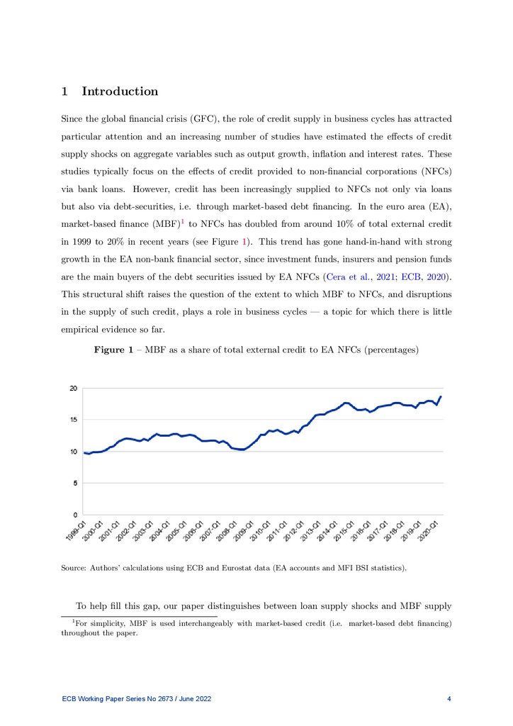
increasingly supplied via debt securities, i.e. through market-based debt financing. In the
euro area (EA), market-based finance (MBF) has doubled from around 10% of total external
credit to NFCs in 1999 to 20% in recent years. This structural shift raises the question of the
extent to which MBF to NFCs, and disruptions in the supply of such credit, plays a role in
explaining business cycles — a topic for which there is little empirical evidence so far.
To help fill this gap, our paper distinguishes between loan supply shocks and MBF supply
shocks, and quantifies their impact on GDP growth in the EA. We do so for the EA as a whole
and also separately for the five largest EA economies, namely Germany, France, Italy, Spain and
the Netherlands.
We draw from a novel quarterly dataset of loan and MBF data for EA NFCs. These data
capture a variety of financing sources for EA NFCs, including financing from various EA sectors
(e.g. bank versus non-bank financing) and from the rest of the world. To conduct the analysis
at country level, we extend the dataset by compiling the same type of data for the five largest
EA countries.
In line with the literature, we use a Bayesian vector autoregression (VAR) model that
incorporates growth in both loans and debt securities, along with four other standard macroeconomic
variables (real GDP growth, inflation, the corporate bond spread and the one-year nominal
interest rate). To identify credit supply shocks, we apply sign restrictions consistent with the
recent macroeconomic literature. To distinguish between the two types of credit supply shocks,
i.e. loan supply shocks and MBF supply shocks, we impose inequality restrictions.
Our results suggest that MBF supply shocks play an important role in explaining GDP
growth in the EA and one that is comparable to that of loan supply shocks. Despite some
differences, MBF supply shocks are found to be important in explaining GDP growth in all five
of the largest EA countries. In Germany and France, where corporate debt markets are relatively
well developed, the explanatory power of MBF supply shocks exceeds that of loan supply shocks.
Their impact on GDP growth in these two countries is also found to be more persistent and
ECB Working Paper Series No 2673 / June 2022
2

4.

stronger than in the three other large EA economies (Italy, Spain and the Netherlands), with
Italy and Spain in particular continuing to rely heavily on bank-based financial systems.
The historical decomposition for the EA also underscores that the two credit supply shocks
explain a large portion of the fall in GDP during the GFC, with loan supply shocks accounting
for slightly more of the GDP fall than MBF supply shocks. By contrast, the impact on GDP
of the two credit supply shocks was less pronounced during the pandemic-induced recession in
early 2020. The MBF supply shock appears to have had an adverse impact on GDP, explaining
around a quarter of the contraction in EA GDP in the first quarter of 2020, whereas this was not
the case for the loan supply shock. The lesser impact of credit supply shocks on GDP growth in
the pandemic-induced recession compared with the GFC is in line with the non-financial origin
of the 2020 recession.
Overall, our findings underline the importance of MBF for EA GDP growth in general
and its adverse effects during crisis periods in particular. Since MBF is mostly provided by
non-bank financial intermediaries, the findings also suggest that their resilience is important
for GDP growth. In this respect, enhancing the macroprudential framework for non-banks
would strengthen the resilience of MBF, while also supporting GDP growth. For instance, in
March 2020 non-banks shed assets on a large scale and market-based debt financing dried up,
while NFCs continued to benefit from loans and credit lines provided by banks. Several factors
supported the flow of bank credit to NFCs during the turmoil, including government guarantees
and moratoria on loans, together with liquidity provided to banks by central banks. Nevertheless,
the regulatory reforms of the banking system after the GFC, including macroprudential measures,
also made banks more resilient to shocks. From this perspective, our results call for more
regulatory attention to be paid to non-banks going forward.
ECB Working Paper Series No 2673 / June 2022
3

5.

1
Introduction
Since the global financial crisis (GFC), the role of credit supply in business cycles has attracted
particular attention and an increasing number of studies have estimated the effects of credit
supply shocks on aggregate variables such as output growth, inflation and interest rates. These
studies typically focus on the effects of credit provided to non-financial corporations (NFCs)
via bank loans. However, credit has been increasingly supplied to NFCs not only via loans
but also via debt-securities, i.e. through market-based debt financing. In the euro area (EA),
market-based finance (MBF)1 to NFCs has doubled from around 10% of total external credit
in 1999 to 20% in recent years (see Figure 1). This trend has gone hand-in-hand with strong
growth in the EA non-bank financial sector, since investment funds, insurers and pension funds
are the main buyers of the debt securities issued by EA NFCs (Cera et al., 2021; ECB, 2020).
This structural shift raises the question of the extent to which MBF to NFCs, and disruptions
in the supply of such credit, plays a role in business cycles — a topic for which there is little
empirical evidence so far.
Figure 1 – MBF as a share of total external credit to EA NFCs (percentages)
Source: Authors’ calculations using ECB and Eurostat data (EA accounts and MFI BSI statistics).
To help fill this gap, our paper distinguishes between loan supply shocks and MBF supply
1
For simplicity, MBF is used interchangeably with market-based credit (i.e. market-based debt financing)
throughout the paper.
ECB Working Paper Series No 2673 / June 2022
4

6.

shocks and quantifies their impact on the EA real economy. We do so for the EA as a whole and
also separately for the five largest EA economies, namely Germany, France, Italy, Spain and the
Netherlands.
To do so, we use a novel quarterly dataset on loan and market-based debt financing provided
to EA NFCs, constructed internally in the ECB (Cera et al., 2021; ECB, 2020). The data are
compiled from ECB and Eurostat sources: euro area accounts (EAA) and monetary financial
institution balance sheet items (MFI BSI) statistics. To conduct the country-level analysis, we
extend the dataset by compiling the same type of data for the five largest EA countries.
Throughout the paper, we use a Bayesian vector autoregression (VAR) model with six
variables: nominal loan and debt securities growth, real GDP growth, inflation, the corporate
bond spread and the one-year nominal interest rate. Abstracting from the novelty of two types
of credit supply shock, our model draws on existing literature to identify the various shocks.
It uses the sign restrictions approach in line with Faust (1998), Canova and De Nicolo (2002),
Uhlig (2005) and Rubio-Ramirez et al. (2010), and follows Eickmeier and Ng (2015), Gambetti
and Musso (2017) and Mumtaz et al. (2018) to distinguish credit supply shocks from other
shocks. Specifically, an unexpected positive credit supply shock (loan or MBF supply shock)
is associated with higher output growth, higher inflation, a higher one-year interest rate and a
lower spread. A positive loan supply shock increases loan growth, while a positive MBF supply
shock increases debt securities growth.
To distinguish between a loan supply shock and a MBF supply shock, we propose a novel
identification scheme with inequality restrictions in line with Peersman (2005). Specifically, the
contemporaneous response of loans (debt securities) is assumed to be the largest for the loan
(MBF) supply shock.
We estimate the model using quarterly data from the first quarter of 1999 to the second
quarter of 2020, paying particular attention to the extraordinary events caused by the coronavirus
(COVID-19) pandemic. In the baseline model, we exclude the two quarters of 2020 from the
sample in view of the very specific nature and extraordinary magnitude of the COVID-19 shocks.
However, to estimate the impact of loan and MBF supply shocks during the pandemic-induced
recession in early 2020, we incorporate a stochastic volatility framework into our Bayesian VAR
model in the spirit of Lenza and Primiceri (2020) and Carriero et al. (2021).
Our results suggest that both credit supply shocks have a significant impact not only on the
EA economy as a whole, but also on each of the five largest EA economies. Specifically, for
ECB Working Paper Series No 2673 / June 2022
5

7.

the EA as a whole, a forecast error variance (FEV) decomposition of GDP growth, inflation,
corporate bond spread and interest rate suggests that loan and MBF supply shocks make a
comparable contribution to explaining variations in these variables. Looking at GDP growth in
the five largest EA economies, we find that the MBF supply shock contributes more than the
loan supply shock in Germany and France, but less in Italy and Spain. In the Netherlands, loan
supply shock makes a marginally larger contribution.
Related literature. Our paper contributes to and combines two strands of literature. It
adds to the relatively large strand of literature on the impact of credit supply shocks on the real
economy by introducing and evaluating a new type of credit supply shock: a MBF supply shock.
Moreover, it significantly expands the recently emerging literature on the economic importance
of the growing share of market-based and/or non-bank financing in the EA. In particular, it is
the first paper – to our knowledge – that evaluates the relative importance of loan and MBF
supply shocks on business cycles in the EA and the five largest EA countries.
Regarding the strand of literature on the impact of credit supply shocks on the real economy,
a number of papers, including Gilchrist et al. (2009), Tamási et al. (2011), Abildgren (2012),
Houssa et al. (2013), Bijsterbosch and Falagiarda (2014), Barnett and Thomas (2014), Gilchrist
and Mojon (2018) and Mumtaz et al. (2018), analyse general credit supply shocks. Other authors
study the role of credit supply shocks, in particular bank loan supply, in private non-financial
sectors (see, for example, Hristov et al., 2012; Moccero et al., 2014; Eickmeier and Ng, 2015;
Gambetti and Musso, 2017). To identify credit supply shocks, most of these papers impose sign
restrictions on impulse responses in a VAR framework.
Our paper follows a similar approach and is most related to recent papers by Eickmeier and
Ng (2015), Gambetti and Musso (2017) and Mumtaz et al. (2018). Specifically, Eickmeier and
Ng (2015) use a global VAR (GVAR) model to study the impact of US credit supply shocks
on the US economy and other economies for the period 1983-2009. Using a broad measure of
real private credit, the credit supply shocks are identified based on the theoretically motivated
contemporaneous sign restrictions. In brief, a negative credit supply shock contemporaneously
decreases or has no effect on GDP or the volume of credit (≤ 0). At the same time, the volume
of credit is restricted to decrease more than GDP. The corporate bond rate, the spread between
corporate bond and long-term government bond rates, and the spread between corporate bond
and short-term interest rates are restricted to increase or not be affected at all (≥ 0). The
authors find that negative US credit supply shocks have a strong negative impact on GDP,
ECB Working Paper Series No 2673 / June 2022
6

8.

not only in the US economy but also in other economies. Specifically, US credit supply shocks
are estimated to contribute around 20% to a one-year-ahead FEV of output in the United
States and 10% to the FEV of output in the EA and United Kingdom. Similarly, Gambetti
and Musso (2017) use a VAR model that incorporates loans to the non-financial private sector
and a composite lending rate and then identify credit supply shocks by using sign restrictions
consistent with recent macroeconomic literature. To identify a loan supply shock, the authors
assume that an expansionary shock leads to an increase in real GDP, inflation, the short-term
interest rate and the loan volume and to a decrease in the lending rate.2 Gambetti and Musso
(2017) find that loan supply shocks have significant effects in all three areas analysed (the
EA, the United Kingdom and the United States) for the period 1980-2011, with the impact
increasing towards the end of the sample. Loan supply shocks are found to explain about
16%-21% of the variance of real GDP growth and appear to be the most important during
recessions. In their baseline model, Mumtaz et al. (2018) use a structural VAR for the US
economy, including five endogenous variables (GDP growth, CPI inflation, lending growth to
households and private NFCs, spread and three-month T-bill) with sign restrictions in the spirit
of Gertler and Karadi (2011), together with a constraint on the FEV. The sign restrictions are
in line with the aforementioned papers. Similarly to Gambetti and Musso (2017), the authors
find that credit supply shocks were important during the GFC, accounting for around 50% of
the decline in output growth in the United States.
With respect to the literature on the growing share of market-based and non-bank financing
in the EA, Aldasoro and Unger (2017) use a VAR framework to compare flows of bank loans with
flows of other sources of external financing (equity, debt securities and loans from non-banks) to
the non-financial private sector in the EA (NFCs, private households and non-profit institutions
serving households). Bank loan shocks and other external financing shocks are distinguished
by the substitution assumption where an adverse bank loan supply shock decreases the flow of
bank loans and increases the flow of other sources of financing. We, in contrast, distinguish the
two credit supply shocks by inequality restrictions, which has the advantage of letting the data
decide whether the two types of financing sources are complements or substitutes. In addition,
instead of a relatively broad category of ”types of financing other than bank loans”, we use more
granular measures of sources of financing to the non-financial private sector. The measures are
2
These authors identify four shocks: a loan supply shock,an aggregate supply shock, an aggregate demand
shock and a monetary policy shock.
ECB Working Paper Series No 2673 / June 2022
7

9.

either activity-based (loans versus debt securities in the baseline model) or entity-based (bank
versus non-bank debt financing in the robustness checks).
The rest of the paper is organised as follows. Section 2 describes the construction of our
dataset and the stylised facts about loans and MBF provided to EA NFCs. Section 3 introduces
the model, while Section 4 presents the results of the baseline EA model and the main findings
for each of the five largest EA economies, including a number of robustness checks. Finally,
Section 5 presents our concluding remarks.
2
Data
We use a novel dataset on external credit provided to EA NFCs, which includes data on
both loans and MBF (i.e. marketable debt securities as opposed to loans). The dataset was
constructed internally in the ECB (Cera et al., 2021; ECB, 2020) and covers the period from the
first quarter of 1999 to the second quarter of 2020. The dataset is built from ECB and Eurostat
sources, specifically the EAA and MFI BSI statistics.3 It contains information on various sources
of debt financing to NFCs, including debt financing from EA sectors and the rest of the world.
Thanks to the quarterly frequency, we can combine these data in estimations with other standard
macroeconomic variables, such as output and inflation, in a VAR framework.
In our baseline model specification, we use two baseline measures of external debt financing to
NFCs: (i) loans to EA NFCs and (ii) MBF to EA NFCs. Loans to EA NFCs include loans from
EA banks, loans from EA non-bank financial entities (investment funds, insurance corporations
and pensions funds, other financial institutions (OFIs)) and loans from the rest of the world.
Three issues about this choice are worth pointing out. First, loans from EA NFCs to EA NFCs
are not included because there is no breakdown between intra-group and extra-group loans, and
we expect most of these loans to be intra-group loans in line with Cera et al. (2021) and ECB
(2020). Second, regarding loans from OFIs, these entities can belong to banking groups or be set
up and owned by NFCs. The former case is likely to be external financing, while the latter case
is likely to be intra-group NFC financing. Since there is no information available to distinguish
between the external and internal nature of OFI financing, we first calculate two measures of
3
Since we extend the dataset to country-level data for the five largest EA countries, slightly different to Cera
et al. (2021) and ECB (2020), we do not use data on non-retained securitised loans from the financial vehicle
corporation statistics. However, the volumes of non-retained securities loans are fairly small compared with the
volumes of other sources of debt financing to NFCs.
ECB Working Paper Series No 2673 / June 2022
8

10.

loan volume – one with and one without OFI loans – and then use the average of two measures.
Third, since there is no sector breakdown for loans to EA NFCs from the rest of the world, we
include all foreign loans in our baseline loan measure. Given that about 85% of total financing
to EA NFCs is provided by EA sectors, this assumption is unlikely to significantly affect our
results. Regarding MBF to EA NFCs, our baseline measure refers to marketable debt securities
issued by EA NFCs, regardless of the holder sector. Hence, these debt securities can be held
by both EA sectors (MFIs, investment funds, OFIs, insurance corporations and pensions funds,
and non-financial sectors) and the rest of the world.
In addition to the distinguishing between loans and MBF based on activity, the dataset also
allows us to determine the entity that provides the funding. In particular, we can distinguish
between funding provided by the non-bank financial sector (insurance corporations and pension
funds, investment funds and OFIs) and that provided by the banking sector (MFIs). Since most
loans are granted by banks and most debt securities are held by non-banks, the entity-based
distinction yields two measures of external NFC financing (bank and non-bank financing) that
are similar – but not identical – to our two activity-based baseline measures (loans and MBF).
We use these alternative measures for robustness checks rather than in our baseline model
specification because their construction is subject to a number of limitations and assumptions.
First, since the sector breakdown is generally available only within the EA, the measures are
limited to NFC financing provided by EA banks and non-banks, while omitting financing from
the rest of the world. Second, the time series for the breakdown of debt securities holdings
by holding sector only start at the fourth quarter of 2013. Therefore, we follow Cera et al.
(2021) and ECB (2020) to backcast the sector breakdown to the first quarter of 1999. We do
so by splitting the time series for debt securities held by all EA sectors in proportion to the
first sectoral distribution available (i.e. the sector breakdown in the fourth quarter of 2013).
This method thus relies on the relatively strong assumption that the sector breakdown remained
constant between the first quarter of 1999 and the fourth quarter of 2013. Third, in line with
Cera et al. (2021) and ECB (2020), we apply a special treatment to isolate the debt securities
held by money market funds (MMFs), since MMFs are included in the fourth quarter of 2013
under the MFI sector but are typically considered non-bank financial intermediaries. To break
down MFI securities into those held by (commercial) banks and those held by MMFs, we use
the MFI BSI statistics, where such breakdown is available as of the first quarter of 2006. For the
data from the first quarter of 2006 onwards, we split the MFI holdings of NFC debt securities
ECB Working Paper Series No 2673 / June 2022
9

11.

in proportion to the data available in the MFI BSI statistics. For the data between the first
quarter of 1999 and the fourth quarter of 2005, we make the split in proportion to the first
quarter of 2006 (sub)sectoral breakdown.
To investigate the heterogeneity across countries, we build the same type of measures for the
five largest EA countries (i.e. Germany, France, Italy, Spain and the Netherlands) using the same
sources and techniques described above. In line with the EA dataset, we collect information on
loan and debt securities financing to NFCs in each country, including financing from EA sectors
and the rest of the world.
Figure 2 – MBF as a share of total external credit to NFCs in the EA and five largest EA
economies (percentages)
Source: Authors’ calculations using ECB and Eurostat data (EAA and MFI BSI statistics)..
Figure 2 shows that the importance of MBF to NFCs has increased over time in the EA
and four of the five largest EA economies. Specifically, for the EA as a whole, the MBF share
of total external credit to NFCs doubled from around 10% in 1999 to almost 20% in 2020. Of
the five largest economies, France stands out owing to its large share of MBF, which exceeds
20% throughout most of the sample period. The share increased from 23% in 1999 to more
than 30% in 2020, although this uptrend was interrupted during the GFC, with the MBF share
reaching a trough of around 19% in the first quarter of 2009. Germany’s MBF share recorded a
ECB Working Paper Series No 2673 / June 2022
10

12.

fairly steady increase, almost tripling from 5% in 1999 to around 14% by the end of our sample
period. Similarly, Italy’s MBF share increased steadily over the sample period, from 3% to 13%.
Spain’s MBF share declined from 7% in 1999 to less than 2% in 2005, but then rebounded to
13% in 2020. The Netherlands is the only country where the MBF share did not significantly
increase over our sample period, fluctuating at around 11
Table 1 – Mean and standard deviation of quarter-on-quarter growth in real GDP, NFC loans
and debt securities in three periods
EA GDP growth
EA loan growth
EA debt sec. growth
Full sample
Q1 1999 - Q4 2019
Mean
Std
0.35
0.60
0.94
1.47
1.79
2.33
Sub-sample
Q1 1999 - Q4 2008
Mean
Std
0.45
0.55
1.65
1.07
1.95
2.32
Sub-sample
Q1 2009 - Q4 2019
Mean
Std
0.25
0.63
0.30
1.49
1.65
2.35
DE GDP growth
DE loan growth
DE debt sec. growth
0.33
0.66
1.85
0.87
1.47
5.83
0.32
0.65
2.66
0.75
1.35
5.12
0.34
0.67
1.13
0.97
1.59
6.37
FR GDP growth
FR loan growth
FR debt sec. growth
0.36
1.12
1.57
0.48
1.30
3.28
0.45
1.69
1.14
0.51
1.43
3.49
0.28
0.61
1.96
0.44
0.92
3.06
IT GDP growth
IT loan growth
IT debt sec. growth
0.10
0.74
2.48
0.68
1.67
5.86
0.23
1.99
3.24
0.73
1.43
6.86
-0.01
-0.38
1.81
0.62
0.92
4.79
ES GDP growth
ES loan growth
ES debt sec. growth
0.46
1.39
2.21
0.68
3.12
6.79
0.78
4.15
1.70
0.51
1.98
8.79
0.19
-1.06
2.65
0.70
1.44
4.38
NL GDP growth
NL loan growth
NL debt sec. growth
0.40
1.00
0.97
0.67
1.42
5.66
0.55
1.29
1.28
0.55
1.48
4.47
0.26
0.74
0.68
0.74
1.32
6.58
Source: Authors’ calculations using ECB and Eurostat data (EAA and MFI BSI statistics)..
In Table 1, we provide information on the mean and variance for quarter-on-quarter NFC loan
and debt securities growth and real GDP growth in the EA and the five largest EA economies
in three time windows: full sample (from the first quarter of 1999 to the fourth quarter of 2019)
and two sub-samples (from the first quarter of 1999 to the fourth quarter of 2008 and from the
first quarter of 2009 to the fourth quarter of 2019). Growth is found to be more volatile in MBF
(debt securities) than loans, both in the EA and at country level. This holds regardless of the
sample period. Both debt financing series are also substantially more volatile than real GDP
ECB Working Paper Series No 2673 / June 2022
11

13.

growth. The EA’s lacklustre GDP growth post-2009 is associated with weak growth in both
loans and MBF, with average growth falling from 1.65% in the period 1999-2008 to 0.3% in
2009-2019 for loans and from 1.95% to 1.6% for MBF. However, the dynamics of debt financing
to NFCs is heterogeneous across countries. Loan growth in the post-2009 period is weaker in
most economies, except Germany, where it remains almost the same in both sub-samples. In
Italy and Spain, loans to NFCs fall on average in the 2009-2019 sample period (negative growth
rate of 0.38% and 1.06% respectively). The growth of MBF accelerates in the post-2009 period
in Spain and France, but slows in Germany, Italy and the Netherlands.
Our model includes a number of other macroeconomic variables (see Section 3). EA and
country-specific data on GDP growth and inflation are taken from Eurostat. Corporate bond
spreads for the EA, Germany, France, Italy and Spain are taken from Gilchrist and Mojon (2018),
while the corporate bond spread data for the Netherlands are from internal ECB calculations.
One-year interest rates are proxied by one-year government bond yields for the EA and each
country, which are taken from Datastream. The advantage of using a longer-term rate than the
ECB policy rate is that it incorporates the impact of forward guidance and hence remains a
valid measure of monetary policy stance during the period, while the policy rate is constrained
by the effective lower bound (Jarociński and Karadi, 2020).
3
Model
To estimate the impact of credit supply shocks, we follow the literature and use a VAR model
as follows:
A0 Xt = B0 +
q
X
Bi Xt−i + t
(1)
i=1
where Xt is the vector of six endogenous variables: NFC nominal loan growth, NFC nominal
debt securities growth, real GDP growth, inflation, the corporate bond spread and the one-year
nominal interest rate. For other notations, q is the lag length,B0 deterministic terms, Bi a
6 × 6 matrix of parameters, A0 a 6 × 6 matrix of parameters capturing the contemporaneous
relationships between the endogenous variables, and t a 6 × 6 vector of orthogonal structural
shocks with a Gaussian distribution of mean zero and identity covariance matrix.
ECB Working Paper Series No 2673 / June 2022
12

14.

The reduced-form representation implied by the structural model (1) is
Xt = C0 +
q
X
Ci Xt−i + ut
(2)
i=1
−1
−1
where C0 = A−1
0 B0 , Ci = A0 Bi and ut = A0 t . It is known that the reduced-form estimation
does not provide enough information to identify even one column of A0 . To overcome this, we
follow Faust (1998), Canova and De Nicolo (2002), Uhlig (2005) and Rubio-Ramirez et al. (2010)
and apply sign restrictions for identifications. Specifically, to identify credit supply shocks we
follow similar sign restrictions to those in Mumtaz et al. (2018), Gambetti and Musso (2017)
and Eickmeier and Ng (2015). We summarise all these restrictions in Table 2.
Table 2 – Contemporaneous sign restrictions in the baseline model
GDP growth
Loan supply shock
<= 0
MBF supply shock
<= 0
Inflation
<= 0
<= 0
Spread
>= 0
>= 0
1Y interest rate
<= 0
<= 0
Loan growth
<= 0
Debt securities growth
Other restrictions
<= 0
(absolute) response of loans growth
is largest
(absolute) response of debt
securities growth is largest
Note: The table lists signs of responses of endogenous variables (in the first column) to negative loan and MBF
supply shocks respectively.
Our main assumptions for the contemporaneous sign restrictions are standard. An unexpected
negative credit supply shock (loan or MBF) is associated with non-positive responses of GDP
growth, inflation and the one-year interest rate, and with non-negative responses in the spread.
Moreover, a negative loan supply shock also leads to a contemporaneous non-positive impact
on loan growth, while a negative MBF supply shock leads to a non-positive response in debt
securities growth.
Nevertheless, these sign restrictions do not distinguish between a loan and an MBF supply
shock. We therefore impose additional inequality restrictions along the lines of Peersman (2005)
by assuming that loan growth has the largest response (in absolute terms) to a loan supply
shock compared with the other variables. Similarly, we assume that debt securities growth has
ECB Working Paper Series No 2673 / June 2022
13

15.

the largest response to an MBF supply shock compared with the other variables.
In line with the literature on sign-identified VAR models, we apply Bayesian methods for
inference. We set priors using dummy observations, as in Banbura et al. (2010). Then, we
use a Gibbs sampling approach and draw A−1
0 directly in each iteration by using the efficient
algorithm proposed by Rubio-Ramirez et al. (2010). In a nutshell, given the draw of var(ut ) =
Ω, the Cholesky decomposition of Ω = Ã00 Ã0 is computed. This matrix Ã0 is multiplied by
an orthogonal rotation matrix Qt , generating a draw of A−1
0 = Qt Ã0 . We only retain those
draws that satisfy the aforementioned sign and inequality restrictions and estimate the impulse
responses to loan and MBF supply shocks.
In addition to the baseline model, we consider a number of alternative identification schemes
and robustness checks. For instance, we apply the inequality restrictions to the FEV decomposition
instead of to the impulse response (see subsection 4.3). In our baseline model specification, we
use two lags of endogenous variables, but we test the robustness of this choice in the online
appendices A.1.1 and A.1.2. We also use an entity-based rather than activity-based measure
of NFC funding (see Section 2 and subsection 4.4). Furthermore, in our baseline analysis, we
exclude from the sample the early 2020 pandemic-induced recession, given the different nature
and extraordinary magnitude of the COVID-19 shocks. However, to study the role of the two
credit supply shocks during the pandemic-induced recession, we extend our VAR model to
incorporate stochastic volatility in order to account for the exceptionally large shocks in early
2020, following Lenza and Primiceri (2020) and Carriero et al. (2021), while maintaining the
identification scheme with sign and inequality restrictions, as discussed above (see subsection
4.5).
4
Results
This section presents the estimates of loan and MBF supply shocks on different economic
variables including output, inflation, corporate bond spread, one-year interest rate, loan growth
and debt securities growth. We first present the baseline results for the EA (subsection 4.1) and
the five largest EA countries (subsection 4.2), and then extend the discussion in several important
dimensions. In particular, we perform robustness checks by controlling for monetary policy
shocks, using a richer identification scheme of shocks (identifying five different shocks), using
the pre-unconventional monetary policy sample (until the second quarter of 2014), excluding
ECB Working Paper Series No 2673 / June 2022
14

16.

restrictions on interest rate and inflation, and using alternative inequality restrictions (subsection
4.3). We extend our analysis to investigate bank versus non-bank credit supply shocks instead of
loan versus MBF supply shocks (subsection 4.4). Finally, we extend our analysis by incorporating
stochastic volatility framework into our Bayesian VAR model to deal with the COVID-19-related
sample and then analyse the impacts of loan and MBF supply shocks in the context of the
COVID-19 crisis (subsection 4.5).
4.1
4.1.1
Baseline
Impulse responses
We start by analysing the baseline results for the EA model. Figure 3 presents the impulse
responses of the EA variables to a loan shock, equivalent to a 1% decrease in loan growth.4 This
shock has a significant negative impact on the EA economy. More specifically, output, i.e. the
cumulative response of output growth, decreases by nearly 0.2% on impact, reaches a trough of
-0.4% in the third quarter, and then gradually returns to zero. The impact is short lasting (for
a year) and then becomes insignificant. At the same time, price, i.e. the cumulative response of
inflation, decreases gradually, but appears long lasting and reaches -0.4% after five years. The
corporate bond spread increases by 0.12% but this is short-lived. The interest rate appears to
follow a Taylor rule-based reaction function, which falls when both output and price decrease.
The rate reduction lasts slightly more than two years, reaching a trough of -0.3 percent after a
year. Such a slow response by the interest rate reflects the persistent decline in prices. Finally,
we capture an increase in debt securities growth on impact, indicating a possible substitution
effect, although it is insignificant. We also observe a decline in MBF growth after two years
which partly reflects the decrease in credit demand due to output contraction.
Figure 4 presents the impulse responses of EA variables to a negative MBF shock, equivalent
to a 1% decrease in debt securities growth. The shock decreases EA output by about 0.3% after
a year. This result is short lasting and significant for up to six quarters. At the same time, the
price decreases gradually, which remains long lasting. The corporate bond spread increases by
0.11% and then returns to zero. Compared with the loan supply shock, the interest rate responds
by a smaller reduction of ten basis points, which can be explained by smaller decreases in output
4
As shown in online appendix A.1.3, our results are almost identical when additionally imposing an
orthogonality condition on two credit supply shocks, i.e. we only retain the draws of the two credit supply
shocks without a statistically significant correlation.
ECB Working Paper Series No 2673 / June 2022
15

17.

Figure 3 – Impulse responses to a negative 1% loan supply shock
Output
Price
0
0.4
Spread
0.2
-0.1
0.2
0.15
-0.2
0.1
Percent
Percent
Percent
-0.2
0
-0.3
-0.4
0.05
0
-0.4
-0.5
-0.05
-0.6
-0.6
2
4
6
8
10
12
14
16
18
20
-0.1
2
4
6
8
Quarters
10
12
14
16
18
20
2
4
6
8
Quarters
1Y rate
Loan Growth
0
10
12
14
16
18
20
16
18
20
Quarters
MBF Growth
0
0.6
-0.2
0.4
-0.2
-0.4
Percent
Percent
Percent
-0.1
-0.6
-0.8
0.2
0
-0.3
-0.2
-1
-0.4
-1.2
2
4
6
8
10
12
14
16
18
20
Quarters
-0.4
2
4
6
8
10
12
Quarters
14
16
18
20
2
4
6
8
10
12
14
Quarters
Note: Impulse responses to a loan supply shock that reduces (median) loan growth by 1% on impact. The solid
line is the median response and the shaded area represents the 16th and 84th bounds. The responses of output
and prices are the cumulated responses of GDP growth and inflation respectively.
and price in response to the MBF shock. The negative impact lasts for 3.5 years, reaches -0.23%
in the fourth quarter and gradually returns to zero afterwards. Finally, the model also records
a positive response by loan growth on impact in line with a substitution effect, although this
effect is insignificant.
4.1.2
FEV Decomposition
One interesting question is how much of the FEV is accounted for by these credit supply shocks.
The answer is shown in Table 3 which presents the FEV decomposition for one, four and eight
quarters ahead for all six variables in our VAR model: GDP growth, inflation, spread, interest
rate, loan growth and debt securities growth. For the FEV of the first four variables, the
contribution of both loan supply and MBF supply shocks is relatively similar, although with
some noticeable differences. Loan supply shocks appear to have marginally larger explanatory
power for GDP and inflation, especially over the longer horizons (one and two years ahead),
ECB Working Paper Series No 2673 / June 2022
16

18.

Figure 4 – Impulse responses to a negative 1% MBF supply shock
Output
Price
0
Spread
0.2
0.2
0.1
-0.1
0.15
-0.2
0.1
-0.1
-0.2
Percent
Percent
Percent
0
-0.3
0.05
-0.3
-0.4
-0.4
0
-0.5
-0.5
2
4
6
8
10
12
14
16
18
20
-0.05
2
4
6
8
10
12
14
16
18
20
2
4
6
8
10
12
14
Quarters
Quarters
Quarters
1Y rate
Loan Growth
MBF Growth
16
18
20
16
18
20
0
0
0.4
-0.05
0.3
-0.15
-0.2
0.2
Percent
Percent
Percent
-0.1
0.1
0
-0.5
-1
-0.25
-0.1
-0.3
-0.2
-1.5
-0.35
2
4
6
8
10
12
14
16
18
20
2
4
Quarters
6
8
10
12
Quarters
14
16
18
20
2
4
6
8
10
12
14
Quarters
Note: Impulse responses to an MBF supply shock that reduces (median) MBF growth by 1% on impact. The
solid line is the median response and the shaded area represents the 16th and 84th bounds of responses. The
responses of output and prices are the cumulated responses of GDP growth and inflation respectively.
whereas MBF supply shocks have slightly greater explanatory power for the spread.
More specifically, the contribution of a loan supply shock to the FEV of output growth and
inflation is estimated to be about 20% for each, increasing with longer horizons. This shock
contributes 19.5% to the FEV of the spread at the one-quarter horizon, although this decreases
to 14% at the one and two year horizons.
The contribution of MBF supply shocks to output growth is similar at all horizons (about
17%) with a slightly larger contribution in the short term (one-quarter). Their contribution to
inflation is around 14%-15%, smaller than the corresponding contribution of loan supply shock.
The contribution of MBF supply shocks to the FEV of the spread is also found to have significant
explanatory power, equal to 21.8% in the short-run and then decreasing to 15% in a two-year
horizon. MBF supply shocks contribute slightly less than loan supply shocks to the EA interest
rate.
Finally, loan supply shocks explain a large portion of the FEV of loan growth (44% in quarter
1 and 30% after two years) while MBF supply shocks contribute only 10% to this variable.
ECB Working Paper Series No 2673 / June 2022
17

19.

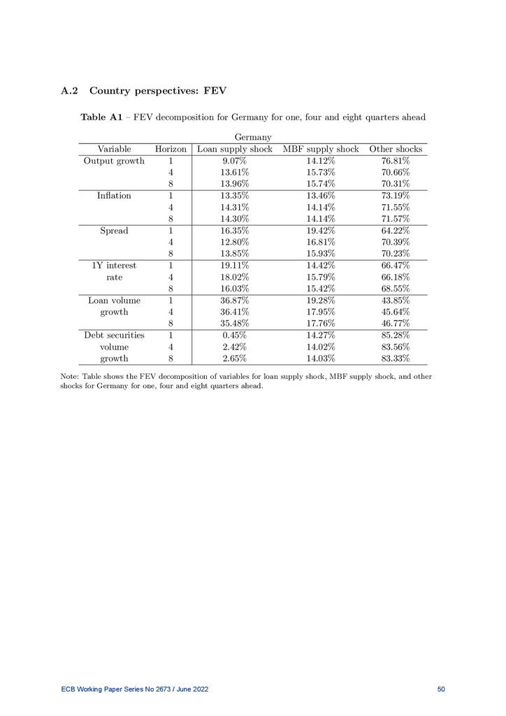
Table 3 – FEV decomposition for one, four and eight quarters ahead
Variable
Output growth
Inflation
Spread
1Y interest
rate
Loan
growth
Debt securities
growth
Horizon
1
4
8
1
4
8
1
4
8
1
4
8
1
4
8
1
4
8
Loan supply shock
18.29%
18.30%
19.08%
18.50%
22.63%
22.12%
19.54%
14.23%
14.86%
20.46%
26.95%
22.46%
43.65%
35.42%
30.53%
3.74%
5.65%
6.61%
MBF supply shock
17.37%
16.77%
16.27%
14.11%
15.00%
15.22%
21.80%
16.28%
15.06%
18.71%
22.71%
21.53%
8.41%
10.44%
11.07%
23.96%
22.26%
21.71%
Other shocks
64.34%
64.93%
64.65%
67.39%
62.37%
62.66%
58.66%
69.50%
70.08%
60.83%
50.34%
56.01%
47.94%
54.15%
58.40%
72.30%
72.09%
71.68%
Note: The table shows the FEV decomposition of variables in the baseline for loan supply shocks, MBF supply
shocks, and other shocks.
Conversely, MBF supply shocks contribute, at up to 24%, significantly more than loan supply
shocks to debt securities growth at the one-quarter horizon.
In total, these two credit supply shocks explain a large amount of the FEV of output growth,
at about 35%, indicating their importance for business cycles as found in the recent literature.
Our results also add new insights to the literature on the relative contributions of the two types
of credit supply shocks.
4.1.3
Historical decomposition
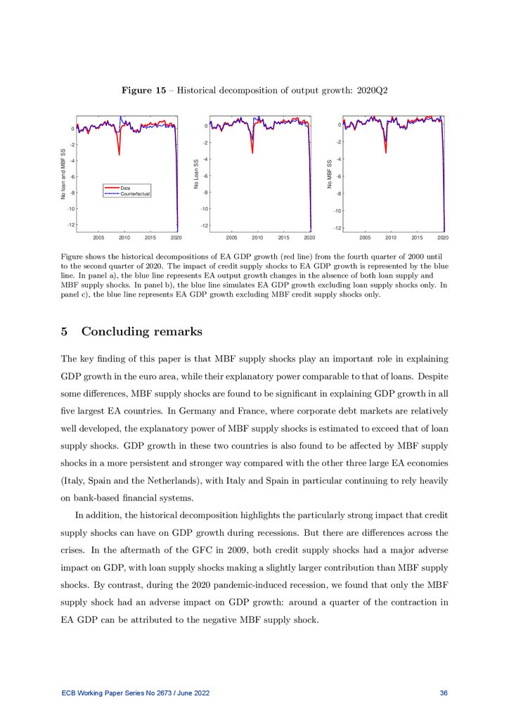
In order to investigate how much these credit supply shocks explain the historically observed
fluctuations in the VAR variables, we perform a historical decomposition and plot this in Figure
5. The impact of credit supply shocks on EA GDP growth, inflation, spread, interest rate,
loan and debt securities growth is represented by the blue lines. The blue lines represent the
counterfactual changes in the absence of both loan supply and MBF supply shocks (first column),
when excluding only loan supply shocks (middle column), and when excluding only MBF credit
supply shocks (third column).
ECB Working Paper Series No 2673 / June 2022
18

20.

The results for the impact on GDP growth (first row in Figure 5) indicate that both credit
supply shocks played an important role, particularly during the recession. In the aftermath of
the GFC in 2009, loan supply shocks accounted for a larger portion of the decrease in GDP than
MBF supply shocks. Specifically, in the fourth quarter of 2009, the two credit supply shocks
accounted for about 50% of the decrease in EA quarter-on-quarter output growth. Loan supply
shocks were responsible for 28% of total contraction and the MBF supply shock for 22%. Our
results for loan supply shocks are in line with those documented in Hristov et al. (2012) and
Gambetti and Musso (2017). Similarly, for the United States, Mumtaz et al. (2018) document
that the trough of the decline in GDP growth in 2009 would have halved in the absence of credit
supply shocks.
Regarding other variables, loan supply shocks had a larger impact on inflation, particularly
before and during the recession in 2008-2009) (second row in Figure 5). MBF supply shocks
also negatively impacted inflation during the recession, but with a smaller magnitude. Spreads
and interest rates (third and fourth rows in Figure 5) were impacted more by loan supply shock
during the recession, while MBF supply shocks seems to have had marginally higher impact on
these variables before 2008 and from 2015 onwards. Finally, the last two rows in Figure 5 reflect
the impact of loan supply shocks on loan growth and of MBF supply shocks on debt securities.
They also show that a significant portion of loan growth and MBF growth is driven by shocks
other than the corresponding supply shocks.
4.2
Country perspectives
This section investigates the impact of the two credit supply shocks at country level. Specifically,
we estimate and identify the shocks with sign restrictions for each of the five largest EA countries:
Germany, France, Italy, Spain, and the Netherlands.
4.2.1
Impulse responses
The impulse responses, as presented in Figure. 6 and Figure 7, are in line with those discussed
for the EA baseline model, i.e. decreases in both credit supply shocks have a negative impact
on economic activity in each of the five economies. Nevertheless, the size of contraction with
respect for each type of credit supply shocks is heterogeneous.
A negative loan supply shock has a large impact on Italy’ and Spain’s output and price
ECB Working Paper Series No 2673 / June 2022
19

21.

Output growth
Figure 5 – Historical decomposition
Data
Counterfactuals
2005
Inflation
Excluding Loan SS
Excluding Loan and MBF SS
0
-1
-2
-3
2010
0
-1
-2
-3
2015
0.5
Excluding MBF SS
0
-1
-2
-3
2005
2010
2015
0.5
0
0
0
-0.5
-0.5
Spread
2010
2015
2005
2010
2015
2
2
2
1
1
1
0
0
0
2005
2010
2015
1Y rate
2015
3
2
1
0
-1
Loan Growth
2010
6
4
2
0
-2
MBF Growth
2005
3
2
1
0
-1
5
5
5
0
0
0
2005
2010
2015
2010
2005
2015
-5
2010
2015
2010
2005
2015
2005
2010
2015
2005
2010
2015
2005
2010
2015
2005
2010
2015
2005
2010
2015
6
4
2
0
-2
2010
2015
-5
-5
2005
2015
3
2
1
0
-1
6
4
2
0
-2
2005
2010
0.5
-0.5
2005
2005
2005
2010
2015
Notes: Figure shows the data (red solid lines) and counterfactual changes (blue dashed lines) when (i) excluding
both loan and MBF supply shocks (“Excluding Loan and MBF SS” in first column); (ii) excluding loan supply
shocks (“Excluding Loan SS” in second column); and (iii) excluding MBF supply shocks (“Excluding MBF SS”
in third column).
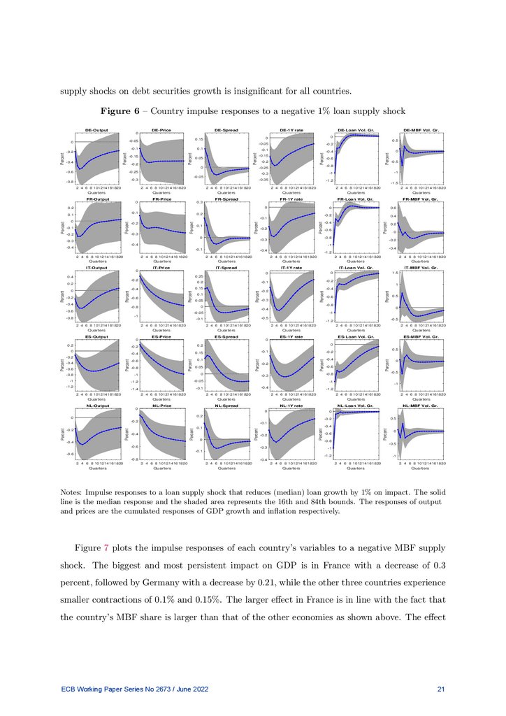
(as seen in the third and fourth rows in Figure 6). A 1% negative loan supply shock causes
Italy’s GDP and price to fall by 0.55% and 0.8% respectively, and Spain’s output and price to
fall by 0.7% and 1.0% respectively. In Germany, France and the Netherlands, however, output
growth decreases by 0.55%, 0.25%, and 0.45% respectively, and prices by 0.18%, 0.3%, and
0.5% respectively. The impact on corporate bond spreads is short lasting and similar in all
countries, increasing the spread by 0.1%-0.15%. The declines in interest rates are larger and
more persistent in Italy and Spain – reflecting the depth of contraction in both output and price
in these two countries – than in Germany, France and the Netherlands. The impact of loan
ECB Working Paper Series No 2673 / June 2022
20

22.

supply shocks on debt securities growth is insignificant for all countries.
Figure 6 – Country impulse responses to a negative 1% loan supply shock
DE-Price
DE-Spread
Percent
Percent
Percent
-0.4
-0.15
-0.2
0.05
0
-0.6
DE-MBF Vol. Gr.
0.5
0.1
-0.1
DE-Loan Vol. Gr.
0
-0.05
-0.2
-0.1
-0.4
-0.15
-0.2
-0.25
-0.25
0
Percent
0
-0.2
DE-1Y rate
0
0.15
Percent
0
-0.05
Percent
DE-Output
-0.6
-0.8
-0.3
-1
-0.35
-1.2
-0.5
-1
-0.05
-0.3
-0.8
-1.5
2 4 6 8 101214161820
2 4 6 8 101214161820
2 4 6 8 101214161820
2 4 6 8 101214161820
2 4 6 8 101214161820
Quarters
Quarters
Quarters
Quarters
Quarters
Quarters
FR-Output
FR-Price
FR-Spread
FR-1Y rate
FR-Loan Vol. Gr.
FR-MBF Vol. Gr.
0
0.3
0
0.2
-0.1
0.1
0.2
2 4 6 8 101214161820
0
0.6
-0.2
0.4
0
-0.2
-1.2
2 4 6 8 101214161820
2 4 6 8 101214161820
2 4 6 8 101214161820
Quarters
Quarters
Quarters
Quarters
Quarters
IT-Price
IT-Spread
IT-1Y rate
Quarters
IT-Loan Vol. Gr.
0
0
-0.1
-0.2
IT-MBF Vol. Gr.
1.5
0.2
0.1
0.05
-0.6
-0.3
0.5
0
-0.4
-0.05
-1
-1
-0.8
-0.6
-0.8
0
-0.8
-0.4
-0.2
Percent
-0.6
-0.4
Percent
Percent
Percent
-0.2
1
0.15
-0.4
0
Percent
-0.2
0.2
-0.5
-0.1
-0.5
-1.2
2 4 6 8 101214161820
2 4 6 8 101214161820
2 4 6 8 101214161820
2 4 6 8 101214161820
2 4 6 8 101214161820
Quarters
Quarters
Quarters
Quarters
Quarters
Quarters
ES-Output
ES-Price
ES-Spread
ES-1Y rate
ES-Loan Vol. Gr.
ES-MBF Vol. Gr.
-0.2
0.2
-0.4
0.15
-0.6
0.1
0
0
0
-0.1
0.05
-0.8
-1
0
-1
-1.2
-0.05
-1.4
-0.1
-1.2
Percent
-0.8
Percent
Percent
Percent
-0.6
0.5
-0.2
-0.2
-0.4
2 4 6 8 101214161820
-0.2
-0.4
Percent
0
0.2
-0.6
-0.8
-0.3
-1
-0.4
-1
2 4 6 8 101214161820
2 4 6 8 101214161820
Quarters
Quarters
Quarters
Quarters
Quarters
Quarters
NL-Output
NL-Price
NL-Spread
NL-1Y rate
NL-Loan Vol. Gr.
NL-MBF Vol. Gr.
0
2 4 6 8 101214161820
0
-0.5
-1.2
2 4 6 8 101214161820
2 4 6 8 101214161820
0
2 4 6 8 101214161820
0
0.2
0
-0.1
0
-0.2
Percent
-0.4
-0.4
-0.4
0.1
Percent
Percent
Percent
-0.2
0.5
-0.2
-0.2
Percent
Percent
2 4 6 8 101214161820
0.25
0.4
Percent
-0.4
-0.4
2 4 6 8 101214161820
0
0
-1
-0.1
2 4 6 8 101214161820
IT-Output
0.2
-0.2
-0.4
-0.4
Percent
-0.6
-0.8
-0.3
-0.3
-0.4
Percent
-0.3
0.1
Percent
-0.2
-0.2
Percent
-0.1
Percent
0
Percent
Percent
-0.1
-0.6
-0.8
0
-0.5
-0.6
-0.3
-1
-0.1
-0.6
-1.2
-0.8
-1
-0.4
2 4 6 8 101214161820
2 4 6 8 101214161820
2 4 6 8 101214161820
2 4 6 8 101214161820
2 4 6 8 101214161820
2 4 6 8 101214161820
Quarters
Quarters
Quarters
Quarters
Quarters
Quarters
Notes: Impulse responses to a loan supply shock that reduces (median) loan growth by 1% on impact. The solid
line is the median response and the shaded area represents the 16th and 84th bounds. The responses of output
and prices are the cumulated responses of GDP growth and inflation respectively.
Figure 7 plots the impulse responses of each country’s variables to a negative MBF supply
shock. The biggest and most persistent impact on GDP is in France with a decrease of 0.3
percent, followed by Germany with a decrease by 0.21, while the other three countries experience
smaller contractions of 0.1% and 0.15%. The larger effect in France is in line with the fact that
the country’s MBF share is larger than that of the other economies as shown above. The effect
ECB Working Paper Series No 2673 / June 2022
21

23.

on price is persistent in all countries, resulting in a decrease of 0.25% in France and around
0.1% in the other four countries. The spread’s response is short-lived and varies from 0.04% to
0.12%, with the strongest impact on France’s corporate bond spread. The decline in interest
rate in Germany, France and the Netherlands remains statistically significant for longer than
in Italy and Spain. Interestingly, for Germany and the Netherlands, we capture a short-lived
but significant increase in loan growth one quarter ahead, indicating a substitution effect. In
summary, we find that the MBF supply shock has a more persistent and stronger impact on
Germany and France than the other three major EA economies.
4.2.2
FEV decomposition
As in the case of the EA baseline, we are interested in the explanatory power of these credit
shocks for the FEV of output growth in the five largest EA economies. As estimated in Table 4,
the contribution of loan supply shocks to the FEV of GDP growth is larger in Italy and Spain
(21%-24% at all horizons) than the other economies. In more detail, it explains 19% at the one
and two-year horizons of the FEV of GDP growth in the Netherlands and up to 14% in Germany
and France.
The contribution of MBF supply shocks to the FEV of GDP growth is estimated to be 15%19% for all countries. They make a larger contribution than loan supply shocks in Germany
and France, while the reverse is true in Italy and Spain. In the Netherlands both credit supply
shocks contributes similarly, with a marginally larger contribution from loan supply shock.
These results are in line with the findings of such authors as Corbisiero and Faccia (2020)
and Gilchrist and Mojon (2018). Corbisiero and Faccia (2020) find that during the European
sovereign debt crisis, higher levels of non-performing loans ratios signalled weakness in banks
balance sheets and thus a limited ability to grant loans, even to sound firms and particularly in
periphery countries, including Italy and Spain. Gilchrist and Mojon (2018) show that bank credit
spreads outperform non-financial credit spreads in explaining economic activity, particularly in
Italy and Spain.
We find similar patterns in the contributions of both shocks to the FEV of other variables
in each economy, as shown in the online appendix A.2. However, there are some interesting
differences. First, both supply shocks make similar contributions to the FEV of inflation in
Germany and the Netherlands, whereas loan supply shock contributes more in France. The
contribution of MBF supply shock to the FEV of the spread is higher in these three countries.
ECB Working Paper Series No 2673 / June 2022
22

24.

Figure 7 – Countries impulse responses to a negative 1% MBF supply shock
DE-Output
0
0
DE-Price
DE-Spread
DE-1Y rate
DE-Loan Vol. Gr.
-0.02
0
0.3
-0.05
-0.25
-0.08
0.2
0.1
-0.5
-1
-0.1
-0.1
-0.3
0.02
-0.06
Percent
-0.08
0.04
Percent
-0.2
Percent
Percent
-0.15
-0.06
Percent
-0.04
-0.04
-0.1
Percent
DE-MBF Vol. Gr.
0
0.06
-0.02
0
-0.12
0
-0.12
-1.5
-0.14
-0.35
2 4 6 8 101214161820
2 4 6 8 101214161820
2 4 6 8 101214161820
2 4 6 8 101214161820
2 4 6 8 101214161820
2 4 6 8 101214161820
Quarters
Quarters
Quarters
Quarters
Quarters
Quarters
FR-Output
FR-Price
FR-Spread
FR-1Y rate
FR-Loan Vol. Gr.
FR-MBF Vol. Gr.
0
0
0
0.2
-0.05
-0.1
0.3
-0.05
0
0.15
-0.1
0.2
-0.2
-0.25
0.1
0.05
-0.15
Percent
-0.15
Percent
-0.3
Percent
-0.2
Percent
Percent
Percent
-0.1
0.1
0
-0.2
-0.5
-1
-0.1
-0.3
-0.4
-0.25
0
-0.2
-0.35
-0.3
2 4 6 8 101214161820
2 4 6 8 101214161820
2 4 6 8 101214161820
Quarters
Quarters
Quarters
Quarters
Quarters
Quarters
IT-Output
IT-Price
IT-Spread
IT-1Y rate
IT-Loan Vol. Gr.
IT-MBF Vol. Gr.
0
2 4 6 8 101214161820
0.06
2 4 6 8 101214161820
0
2 4 6 8 101214161820
0.1
0.05
0
0.04
-0.02
0.02
-0.04
-0.06
0
0.05
Percent
-0.1
-0.1
Percent
-0.05
Percent
Percent
0
Percent
-0.05
Percent
-1.5
0
-0.5
-1
-0.15
-0.15
-0.08
-0.02
-0.05
-1.5
2 4 6 8 101214161820
2 4 6 8 101214161820
2 4 6 8 101214161820
2 4 6 8 101214161820
2 4 6 8 101214161820
Quarters
Quarters
Quarters
Quarters
Quarters
Quarters
ES-Loan Vol. Gr.
ES-MBF Vol. Gr.
ES-Price
ES-Spread
ES-1Y rate
0.08
0
0.2
0.25
0.02
0.06
0
0.04
-0.02
0.2
-0.1
0.02
0
-0.2
-0.02
-0.04
0.1
0.05
-0.06
0
-0.08
-0.05
-0.5
-1
-1.5
-0.1
-0.1
-0.2
2 4 6 8 101214161820
2 4 6 8 101214161820
Quarters
Quarters
Quarters
Quarters
Quarters
Quarters
NL-Output
NL-Price
NL-Spread
NL-1Y rate
NL-Loan Vol. Gr.
NL-MBF Vol. Gr.
2 4 6 8 101214161820
0
0.08
-0.05
-0.05
-0.1
-0.15
Percent
-0.1
-0.15
Percent
Percent
0.06
0.04
0.02
2 4 6 8 101214161820
0.3
-0.02
0.25
-0.04
0.2
-0.06
-0.08
0
0
0.15
0.1
-0.5
-1
0.05
-0.2
-0.2
2 4 6 8 101214161820
Percent
2 4 6 8 101214161820
Percent
0
0
Percent
Percent
-0.1
-0.15
Percent
0
0
0.15
Percent
Percent
Percent
-0.05
0.1
Percent
ES-Output
0.3
2 4 6 8 101214161820
-0.1
-0.02
0
-1.5
-0.12
-0.25
2 4 6 8 101214161820
2 4 6 8 101214161820
2 4 6 8 101214161820
2 4 6 8 101214161820
2 4 6 8 101214161820
2 4 6 8 101214161820
Quarters
Quarters
Quarters
Quarters
Quarters
Quarters
Notes: Impulse responses to an MBF supply shock that reduces (median) MBF growth by 1% on impact. The
solid line is the median response and the shaded area represents the 16th and 84th bounds of responses. The
responses of output and prices are the cumulated responses of GDP growth and inflation respectively.
In Italy and Spain, loan supply shocks explain a larger share of inflation and spread variations.
Regarding interest rates, loan supply shocks explain a larger share of FEV in all countries.
4.2.3
Historical decomposition
We now discuss how much the two credit supply shocks explain the historical observations of
output growth in these economies. Each row of Figure 8 presents the historical decomposition
ECB Working Paper Series No 2673 / June 2022
23

25.

Table 4 – Country results: FEV decomposition for output growth for one, four and eight
quarters ahead
Country
Germany
France
Italy
Spain
Netherlands
Horizon
1
4
8
1
4
8
1
4
8
1
4
8
1
4
8
Loan supply shock
9.07%
13.61%
13.96%
14.01%
13.26%
14.02%
23.78%
21.91%
21.53%
20.95%
24.41%
22.08%
16.31%
18.95%
18.86%
MBF supply shock
14.12%
15.73%
15.74%
15.16%
16.38%
15.80%
19.66%
17.95%
17.19%
16.64%
13.51%
13.41%
16.66%
17.49%
17.08%
Other shocks
76.81%
70.66%
70.31%
70.83%
70.36%
70.18%
56.57%
60.14%
61.27%
62.41%
62.08%
64.50%
67.03%
63.56%
64.05%
Note: The table shows the FEV decomposition of output growth for loan supply shock, MBF supply shock, and
other shocks for five EA countries.
of output in each economy. In line with the EA baseline model, the historical decomposition
highlights the significant impact of both credit supply shocks on GDP growth in all economies,
particularly during the recession.
In all economies, these two shocks explain a large portion of output decline in the aftermath
of the 2009 GFC. In Italy, Spain and the Netherlands, as in the baseline EA model, loan supply
shocks account for a slightly larger portion of the GDP fall compared to MBF supply shocks.
Specifically, in the fourth quarter of 2009, both credit supply shocks cause a decrease of about
1.5% in the quarter-on-quarter output growth of each of these three economies (equivalent to
about 50% of total output contraction). In Italy, Spain and the Netherlands, loan supply shocks
are responsible for drops in output of 0.81%, 0.82%, and 0.95% respectively, and the MBF supply
shocks for 0.68%, 0.73%, and 0.72% of GDP contractions in each country respectively.
The picture is slightly different for Germany and France, where in 2009 both MBF supply
shocks and loan supply shocks lead to a similar drop in output growth. In the fourth quarter
of 2009, the two credit supply shocks account for 41% of total quarter-on-quarter GDP growth
contraction in Germany (-2.12%) and for 36% in the output growth of France (-0.72%). Of the
total impact of credit supply shocks on output contraction, MBF supply shock accounts for 52%
ECB Working Paper Series No 2673 / June 2022
24

26.

in Germany (-1.1%) and 49% in France (-0.35%).
Figure 8 – Country results: historical decomposition of output
0
0
-1
-2
1
0
No MBF SS
1
No loan SS
No loan and MBF SS
DE-Output Growth
1
-1
-2
-1
-2
-3
-3
-3
-4
-4
-4
-5
-5
2005
2010
2015
-5
2005
2010
2015
2005
2010
2015
2005
2010
2015
2005
2010
2015
2005
2010
2015
2005
2010
2015
0.5
0.5
0
0
0
-0.5
-1
-1.5
No MBF SS
0.5
No loan SS
No loan and MBF SS
FR-Output Growth
-0.5
-1
-1.5
-2
2010
2015
-1
-1.5
-2
2005
-0.5
-2
2005
2010
2015
1
1
1
0.5
0.5
0.5
0
-0.5
-1
-1.5
0
No MBF SS
0
No loan SS
No loan and MBF SS
IT-Output Growth
-0.5
-1
-1.5
-0.5
-1
-1.5
-2
-2
-2
-2.5
-2.5
-2.5
2005
2010
2015
2005
2010
2015
ES-Output Growth
0.5
0.5
0
0
-0.5
-0.5
-1
-1.5
No MBF SS
0
-0.5
No loan SS
No loan and MBF SS
0.5
-1
-1.5
-1
-1.5
-2
-2
-2
-2.5
-2.5
-2.5
-3
-3
2005
2010
2015
-3
2005
2010
2015
1
0.5
0.5
0
0
0
-0.5
-0.5
-1
-1.5
-2
-2.5
1
0.5
No MBF SS
-0.5
No loan SS
No loan and MBF SS
NL-Output Growth
1
-1
-1.5
-2
-1
-1.5
-2
-2.5
-2.5
-3
-3
-3
-3.5
-3.5
-3.5
-4
-4
2005
2010
2015
-4
2005
2010
2015
Notes: Figure shows the data (red solid lines) and counterfactual changes (blue dashed lines) when (i) excluding
both loan and MBF supply shocks (“Excluding Loan and MBF SS” in first column); (ii) excluding loan supply
shocks (“Excluding Loan SS” in second column); and (iii) excluding MBF supply shocks (“Excluding MBF SS”
in third column). Each row presents the historical decomposition for each country.
Interestingly, the historical decomposition of Spain’s output (fourth row of Figure 8) captures
the country’s credit boom (positive credit supply shock) before the GFC in 2009, to which both
loan and MBF supply shocks contribute. However, loan supply shock appears to contribute
more than MBF sypply shock to this boom. This result is in line with Borio (2014).
ECB Working Paper Series No 2673 / June 2022
25

27.

4.3
Sensitivity analyses
In our baseline identification scheme, we identify two types of credit supply shocks of interests:
loan supply shocks and MBF supply shocks. To assess the sensitivity of our identification, we
consider several alternative identification schemes. First, we identify both credit supply shocks
while controlling for monetary policy shocks. The latter are identified by sign restrictions,
where a monetary policy shock raises interest rates and spreads, but reduces output growth and
inflation, as documented in Christiano et al. (2010), Smets and Wouters (2007), and Bernanke
et al. (1999). The identification strategy in this analysis is summarised in columns 2-4 of Table
5.
Table 5 – Sensitivity analyses: contemporaneous sign restrictions
GDP growth
Loan sup.
shock
<= 0
MBF sup.
shock
<= 0
Mon. pol.
shock
<= 0
Agg. dem.
shock
<= 0
Agg. sup.
shock
<= 0
Inflation
<= 0
<= 0
<= 0
<= 0
>= 0
Spread
>= 0
>= 0
<= 0
1Y interest rate
<= 0
<= 0
>= 0
Loan growth
<= 0
Debt securities growth
Other restrictions
<= 0
<= 0
response of
loan
volume growth. is
largest
(abs.)
response of
MBF
volume growth. is
largest
(abs.)
Note: Signs imposed on the impulse response on impact of all variables for the case of a contractionary shock
(i.e. a shock causing a decrease in output growth).
Second, we consider an identification strategy similar to that in Gambetti and Musso (2017)
who identify n − 1 shocks for a VAR system of n endogenous variables, and leave one of the
reduced-form residual shock unidentified to act as a buffer and capture the effects of omitted
variables and other shocks which are different from five identified shocks. This expansion is
motivated by Paustian (2007) who argues that identifying other shocks helps identify the shocks
of interest. Specifically, we identify five different shocks: an MBF supply shock, a loan supply
shock, a monetary policy shock, an aggregate demand shock and an aggregate supply shock.
The sign restrictions of three additional shocks are also only imposed on variables on impact
ECB Working Paper Series No 2673 / June 2022
26

28.

and are summarised in Table 5. The monetary policy shock’s restrictions are described above.
An aggregate demand shock leads to the same sign responses of output growth, inflation and
interest rate. These sign responses are the same as those of MBF and loan supply shocks.
However, the inequality restrictions employed (i.e. the response of loans is the largest on impact
(in absolute terms) for loan supply shock and the response of debt securities is the largest on
impact for MBF supply shock) distinguish credit supply shocks and aggregate demand shocks.
It is also worth noting that aggregate demand shocks include credit demand shocks, although
jointly with other types of demand shock. However, we do not identify credit demand shocks
because of the absence of a credible set of sign restrictions to separate credit demand shocks
from other aggregate demand shocks. We assume that aggregate supply shocks lead to different
signs in the responses of output and inflation, therefore allowing us to distinguish credit supply
shocks and other shocks.
Our third sensitivity analysis follows Eickmeier and Ng (2015), who do not employ restrictions
on the responses of inflation and policy interest rates. This approach comes from observations
that with certain theoretical settings, policy rate and inflation responses to a credit supply shock
may have different signs to those of output growth.5 Therefore, with this sensitivity exercise,
we remove the restrictions on inflation and interest rates from our baseline sign restrictions.
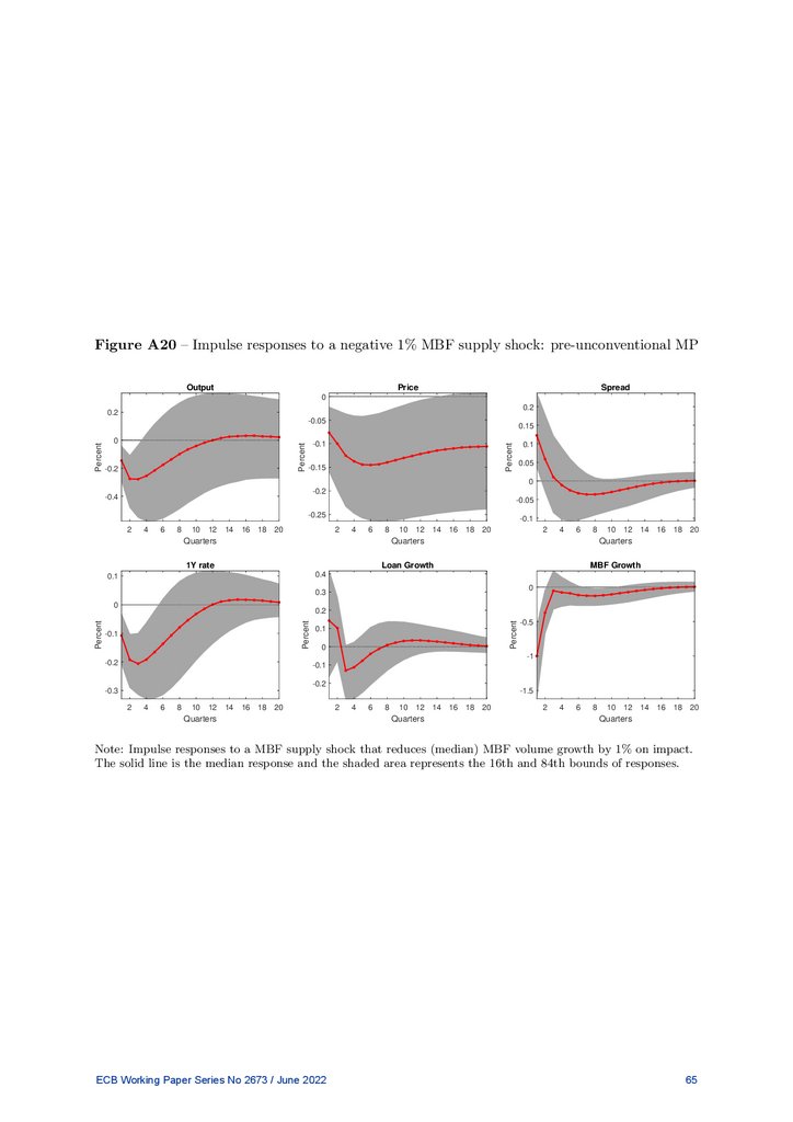
Next, we analyse whether our results are influenced by the introduction of unconventional
monetary policy in the EA. In June 2014, the ECB introduced negative interest rates by lowering
its deposit rate to -0.1% to stimulate the economy. The ECB also started large-scale asset
purchase programmes in September 2014. As a sensitivity check, we exclude the post-second
quarter of 2014 sample from the baseline and re-estimate our model.
Last but not least, we conduct a sensitivity analysis with an alternative inequality restriction
scheme. As discussed in Section 3, instead of setting the inequality restrictions on impulse
responses to distinguish the two credit supply shocks, we place them on the first-quarter FEV
decomposition of loan and debt securities. Specifically, loan supply shock is assumed to explain
more of the FEV of loan growth than MBF supply shock at the first-quarter horizon. Conversely,
the first-quarter FEV of debt securities growth is explained more by MBF supply shock than loan
supply shock. The evidence in Table 3 provides empirical support for this alternative approach
to distinguishing the two supply shocks while retaining other standard sign restrictions on the
5
For instance, Christiano et al. (2010) find that a credit supply shock, i.e. bank funding shock, raises output,
but reduce inflation and policy rates, while Gerali et al. (2010) show that output, inflation and policy rates have
similar signs in response to credit supply shocks.
ECB Working Paper Series No 2673 / June 2022
27

29.

remaining variables.
Figure 9 – Sensitivity analyses: impulse responses to a negative 1% loan supply shock
Output
Price
0
Baseline
Mon. Pol.
Five shocks
No-Rate-Inflation
Pre-20014
FEV
0.4
0.3
-0.1
0.2
-0.2
0.1
Percent
Percent
0
-0.1
-0.2
-0.3
-0.4
-0.3
-0.4
-0.5
-0.5
-0.6
-0.6
2
4
6
8
10
12
14
16
18
20
2
4
6
8
Quarters
10
12
14
16
18
20
Quarters
Notes: Impulse responses to a loan supply shock that reduces (median) loan growth by 1% on impact. The solid
lines are the median responses and the shaded area represents the baseline 16th and 84th bounds of responses.
“Mon. Pol” = controlling for monetary policy shocks; “Five shocks”= an identification with five shocks; “No
Rate-Inflation” = no restrictions on interest rates and inflation; “Pre-2014”= excluding the post-second quarter
of 2014 sample from the analysis; and “FEV” = using inequality restrictions on the variance.
Figure 10 – Sensitivity analyses: Impulse responses to a negative 1% MBF supply shock
Output
Price
0
0.2
-0.05
-0.1
0
-0.15
-0.1
-0.2
Percent
Percent
0.1
-0.2
-0.3
-0.25
-0.3
-0.35
-0.4
-0.4
-0.5
-0.45
Baseline
Mon. Pol.
Five shocks
No-Rate-Inflation
Pre-20014
FEV
-0.5
2
4
6
8
10
12
14
16
Quarters
18
20
2
4
6
8
10
12
14
16
18
20
Quarters
Note: Impulse responses to a MBF supply shock that reduces (median) MBF growth by 1% on impact. The solid
lines are the median responses and the shaded area represents the baseline 16th and 84th bounds of responses.
“Mon. Pol” = controlling for monetary policy shocks; “Five shocks”= an identification with five shocks; “No
Rate-Inflation” = no restrictions on interest rates and inflation; “Pre-2014”= excluding the post-second quarter
of 2014 sample from the analysis; and “FEV” = using inequality restrictions on the variance.
ECB Working Paper Series No 2673 / June 2022
28

30.

Figure 11 – Sensitivity analyses: historical decomposition of output growth
Baseline
0
-1
-2
-3
Data
Counterfactuals
Mon. Pol
2005
Five shocks
No Rate-Inflation
Pre-2014
2010
2015
2010
2015
2010
2005
2015
2010
2015
2010
2005
2015
2010
2015
2010
2005
2015
0
-1
-2
-3
2010
2015
2010
2005
2015
2005
2010
2015
2005
2010
2015
2005
2010
2015
2005
2010
2015
2005
2010
2015
0
-1
-2
-3
2010
2015
0
-1
-2
-3
0
-1
-2
-3
2005
2015
0
-1
-2
-3
0
-1
-2
-3
2005
2010
0
-1
-2
-3
0
-1
-2
-3
2005
2005
0
-1
-2
-3
0
-1
-2
-3
2005
0
-1
-2
-3
2005
0
-1
-2
-3
0
-1
-2
-3
0
-1
-2
-3
0
-1
-2
-3
0
-1
-2
-3
2015
0
-1
-2
-3
2005
FEV
2010
Excluding MBF SS
Excluding Loan SS
Excluding Loan and MBF SS
2005
2010
2015
Notes: Figure shows the data (red solid lines) and counterfactual changes (blue dashed lines) when (i) excluding
both loan and MBF supply shocks (“Excluding Loan and MBF SS” in first column); (ii) excluding loan supply
shocks (“Excluding Loan SS” in second column); and (iii) excluding MBF supply shocks (“Excluding MBF SS”
in third column). The first row shows the baseline decomposition, and the other rows show the decompositions
of alternative sensitivity analyses: “Mon. Pol” = controlling for monetary policy shocks; “Five shocks”= an
identification with five shocks; “No Rate-Inflation” = no restrictions on interest rates and inflation;
“Pre-2014”= excluding the post-second quarter of 2014 sample from the analysis; and “FEV” = using inequality
restrictions on the variance.
Figure 9 shows the impulse responses of output and price to a loan supply shock.6 Controlling
for monetary policy shocks and adopting five-shock identification lead to similar responses.
Removing restrictions on inflation and interest rates leads to a larger fall in output (about 0.5% after a year). The impact is also more persistent than the baseline. Nevertheless, even
6
The impulse responses of all variables to both credit supply shocks, together with the historical decompositions
of all variables for each of four alternative identification schemes separately, can be found in online Appendix A.3.
ECB Working Paper Series No 2673 / June 2022
29

31.

without a restriction on price, its response is in line with the baseline, indicating a decrease of
price in response to a contractionary loan supply shock. The alternative inequality restrictions
on FEV lead to slightly larger responses of output and price. Regarding the pre-unconventional
monetary policy sample, the results show a larger fall in output (about -0.5% after 1.5 years).
In addition, the impact on output and price is less persistent. Despite these differences, we find
that all these point estimates stay in the baseline 16th-84th bounds, therefore corroborating our
findings. We also find that the responses to an MBF supply shock are robust in alternative
sensitivity analyses (see Figure 10). In most cases, the point estimates stay in the baseline
16th-84th bounds.
Table 6 – Sensitivity analyses: FEV decomposition of EA output growth and inflation for one,
four and eight quarters ahead
Model
Baseline
Control for monetary
policy shocks
Five-shock
identification
No restrictions on
interest rate and
inflation
Pre-unconventional
monetary policy
Inequality restrictions
on FEV
Horizon
1
4
8
1
4
8
1
4
8
1
4
8
1
4
8
1
4
8
FEV for EA output growth
loan sup.
MBF sup.
shocks
shocks
18.29%
17.37%
18.30%
16.77%
19.08%
16.27%
17.16%
16.12%
16.95%
15.52%
17.95%
15.23%
15.26%
15.32%
16.03%
15.24%
16.89%
14.88%
17.71%
17.38%
18.73%
19.74%
18.95%
19.16%
18.13%
16.88%
18.17%
14.57%
19.85%
14.02%
19.87%
17.15%
19.52%
16.72%
20.38%
16.21%
FEV for EA inflation
loan sup. MBF sup.
shocks
shocks
18.50%
14.11%
22.63%
15.00%
22.12%
15.22%
17.02%
13.67%
20.71%
14.16%
20.31%
14.42%
16.12%
12.43%
19.66%
13.18%
19.32%
13.53%
18.49%
15.18%
21.28%
15.17%
20.92%
15.65%
21.12%
13.75%
24.43%
13.05%
23.59%
12.86%
20.21%
13.27%
24.07%
14.38%
23.51%
14.64%
Note: Table shows the FEV decomposition of EA output growth and inflation for one, four and eight quarters
ahead.
The historical decomposition shown in Figure 11 also indicates similarity in the roles of loan
and MBF supply shocks in the dynamics of output growth, particularly their crucial role during
the financial crisis. Variance decomposition analysis in Table 6 also corroborates our baseline
findings that both credit supply shocks are important, explaining more than 30% of the FEV
ECB Working Paper Series No 2673 / June 2022
30

32.

of EA output growth and inflation across all horizons. Regarding output growth, in most cases,
loan supply shocks have a larger explanatory power than MBF supply shocks by 2 to 5 percentage
points at the two-year horizon. Without restrictions on interest rate and inflation, MBF supply
shocks contribute slightly more at the one- and two-year horizons by 1 percentage point and
0.2 percentage point respectively. Conversely, we find that loan supply shocks dominate MBF
supply shocks in explaining the FEV of EA inflation in all cases; specifically, at the two-year
horizon, the differences range from 5 percentage points to 10 percentage points.
4.4
EA bank versus non-bank supply shocks
So far our analysis has focused on the distinction between loans and debt securities that are
activity-based. It is well known that loans are mostly granted by banks while non-bank financial
sectors hold the larger portion of debt securities (Cera et al., 2021). Our dataset also allows us to
identify the source of funding based on entity: the share of non-bank financial sector compared
with the banking sector. We therefore extend our analysis to investigate the importance of bank
financing versus non-bank financing. Since the separation of banks and non-banks is available
only within the EA, we perform this robustness check by focusing only on financing from EA
banks and non-banks. EA banks supply about 72% of EA-based total loans and EA non-bank
financial intermediaries supply 90% of EA-based total MBF. This exercise investigates bank
versus non-bank credit supply shocks instead of loan versus MBF supply shocks.
As shown in online Appendix A.4, the impulse responses to a bank credit supply shock are
similar to those in a loan supply shock, although the decline in output is slightly larger in the
former than the latter (-0.5% versus -0.4% one year after the shock). A similar feature is also
seen in the case of a non-bank credit supply shock (-0.4% for a non-bank shock versus -0.3% for
an MBF shock one year after the shock). Table 7 shows that both bank and non-bank supply
shocks are important, explaining more than 30% of the FEV of EA output growth and inflation
across all considered horizons: first quarter, one year and two years. We also find that bank
supply shocks have more explanatory power for output growth and inflation variations than
non-bank supply shocks. The differences in their contributions are similar to those between loan
and MBF supply shocks, as documented in the baseline estimates. These similarities further
corroborate the robustness of our findings.
ECB Working Paper Series No 2673 / June 2022
31

33.

Table 7 – Sensitivity analysis: FEV decomposition of EA output growth and inflation for one,
four and eight quarters ahead
Model
Horizon
Baseline
1
4
8
Banks vs
non-banks
1
4
8
FEV for EA output growth
Loan sup.
MBF sup.
shocks
shocks
18.29%
17.37%
18.30%
16.77%
19.08%
16.27%
Bank sup. Non-bank sup.
shocks
shocks
18.73%
16.99%
18.56%
16.67%
19.93%
16.13%
FEV for EA inflation
Loan sup.
MBF sup.
shocks
shocks
18.50%
14.11%
22.63%
15.00%
22.12%
15.22%
Bank sup. Non-bank sup.
shocks
shocks
19.31%
16.33%
24.18%
16.07%
23.67%
16.19%
Note: The table shows the FEV decomposition of EA output growth and inflation for one, four and eight
quarters ahead.
4.5
2020 episode
In previous analyses, we excluded the 2020 sample to avoid the potential influence of the
extraordinary COVID-19 event on evaluating the average impact of the two credit supply shocks
over the sample. In this section we extend our analysis to investigate the role played by loan and
MBF supply shocks in the context of COVID-19 crisis in the EA. Specifically, we expand the
sample to include both the first and second quarters of 2020 and we deal with the substantially
large shocks by incorporating a stochastic volatility framework into our Bayesian VAR model,
similarly to Carriero et al. (2021) and Lenza and Primiceri (2020).
Methodology with stochastic volatility
We modify the relation between reduced-form residuals and structural shocks as follows:
1/2
ut = Ωt et , et ∼ N (0, I),
(3)
−10
Ωt = A−1
0 H t A0 ,
(4)
where
where Ht is the diagonal matrix of time-varying standard deviation following a random walk in
a log specification and A0 is as described in (1). Furthermore, for shocks identification, we use
the same contemporaneous sign restrictions and inequality restrictions as in the baseline model,
ECB Working Paper Series No 2673 / June 2022
32

34.

as summarised in Table 2.
Results
Figures 12 and 13 show the impulse responses on impact of the EA variables to loan supply and
MBF supply shocks.7 The response of output to a loan supply shock is close to -0.2%, which
is in line with the baseline estimate, therefore corroborating our findings. However, the same
negative loan supply shock would lead to a larger fall in output during the crises, at about -0.3%
in 2009 and -0.4% in 2020. The average response of output to an MBF supply shock is about
-0.1%, which is similar to the baseline response. However, the impact of this shock is magnified
during the crises, to more than -0.2% in 2009 and -0.3% in 2020. The response of price remains
relatively stable with an MBF supply shock, but varies significantly with a loan supply shock.
The larger response of output in the crises under both credit supply shocks is associated with
larger increases in spreads during the crises. This is in line with Gertler and Karadi (2015) who
show the amplifying role of credit spreads in the responses of economic activity to shocks (i.e.,
monetary policy surprises in their paper). Interestingly, we show that the response of interest
rate has weakened since 2015, reflecting the period associated with the effective lower bounds
in the EA.
While the impulse responses analyses are helpful in showing the impacts of these shocks,
they do not reflect the role played by the shocks at every given point in time. For example, did
credit supply shocks contribute to the 2020 recession? Nevertheless, it is interesting to quantify
how much these structural shocks explain the historical decline observed in output in 2020. We
address this question with a historical decomposition analysis. To enhance visualisation, we
present historical decomposition of output growth in Figures 14 and 15, which end at the first
quarter of 2020 and the second quarter of 2020, respectively. In line with the baseline model,
the model with stochastic volatility further highlights the crucial roles played by both credit
supply shocks in GDP growth, particularly during the recessions. In the GFC in 2009, loan
supply shocks accounted for a slightly larger portion of the decrease in GDP compared with the
MBF supply shock, which confirms the baseline results. Nevertheless, when allowing for the
stochastic volatility, both credit supply shocks are found to cause a larger contraction in EA
output growth (Figure 14, reflecting the larger impacts of these two shocks during the crises as
shown in the impulse responses in Figures 12 and 13. Given the limited sample for a stochastic
7
See online appendix A.5 regarding impulse responses for four periods ahead.
ECB Working Paper Series No 2673 / June 2022
33

35.

Figure 12 – Impulse responses to a negative 1% loan supply shock: period 1
Output
0
Price
0
Spread
0.3
-0.1
-0.2
0.25
-0.2
0.2
-0.4
-0.3
0.15
-0.6
-0.4
0.1
-0.5
-0.8
2000
2005
2010
2015
2020
1Y rate
0
-0.6
2000
0.05
2005
2010
2015
0
2000
2020
2005
Loan Growth
0
2010
2015
2020
2015
2020
MBF Growth
0.8
-0.1
0.6
-0.5
0.4
Percent
-0.2
-1
-0.3
-0.4
0.2
0
-0.2
-1.5
-0.4
-0.5
2000
2005
2010
2015
2020
2000
2005
2010
2015
2020
2000
2005
2010
Notes: Impulse responses to a loan supply shock that reduces (median) loan growth by 1% on impact. The solid
line is the median response and the shaded area represents the 16th and 84th bounds of responses.
Figure 13 – Impulse responses to a negative 1% MBF supply shock: period 1
Output
0
Price
0
Spread
0.35
-0.1
0.3
-0.2
-0.05
0.25
-0.3
0.2
-0.4
0.15
-0.1
0.1
-0.5
0.05
-0.6
2000
-0.15
2005
2010
2015
2020
2000
2005
1Y rate
0
2010
2015
0
2000
2020
Loan Growth
2005
2010
2015
2020
2015
2020
MBF Growth
0
0.6
-0.05
0.4
-0.5
Percent
-0.1
0.2
-0.15
-1
0
-0.2
-0.2
-1.5
-0.25
2000
2005
2010
2015
2020
2000
2005
2010
2015
2020
2000
2005
2010
Notes: Impulse responses to a MBF supply shock that reduces (median) MBF growth by 1% on impact. The
solid line is the median response and the shaded area represents the 16th and 84th bounds of responses.
ECB Working Paper Series No 2673 / June 2022
34

36.

volatility framework, these results should be interpreted with caution. However, the findings
further reinforce the baseline results regarding the large impact of these credit supply shocks on
business cycles.
Figure 14 – Historical decomposition of output growth: Q1 2020
1.5
1
1
No Loan SS
0
-0.5
-1
-1.5
0
0
-0.5
-0.5
No MBF SS
0.5
No loan and MBF SS
0.5
0.5
-1
-1.5
-2
-1
-1.5
-2
-2
-2.5
-2.5
Data
Counterfactual
-2.5
-3
-3
-3
-3.5
-3.5
-4
2005
2010
2015
2020
-0.9
-3.5
2005
2010
2015
2020
2005
2010
2015
2020
Notes: Figure shows the historical decompositions of EA GDP growth (red line) from the fourth quarter of 2000
until to the first quarter of 2020. The impact of credit supply shocks to EA GDP growth is represented by the
blue line. In panel a), the blue line represents EA output growth changes in the absence of both loan supply and
MBF supply shocks. In panel b), the blue line simulates EA GDP growth excluding loan supply shocks only. In
panel c), the blue line represents EA GDP growth excluding MBF credit supply shocks only.
By contrast, it is interesting to note that the impact on GDP of both credit supply shocks
was less pronounced during the pandemic-induced recession in early 2020. The MBF supply
shock appears to have had an adverse impact on GDP (explaining a quarter of the decrease in
GDP), but this is not the case for the loan supply shock. These results likely reflect the greater
impact of the March 2020 market turmoil on non-bank financial intermediaries than on banks.
Specifically, the banking system did not cut funding to the real economy and continued to provide
credit lines, thus helping to mitigate the contraction in GDP, whereas bonds issuance almost
froze. Furthermore, in the second quarter of 2020 when the markets stabilised after significant
interventions by monetary and fiscal authorities, MBF supply and loan supply shocks had a
negligible impact on the decrease in GDP as bank and non-bank credit started to finance the
real economy again (Figure 15). This large contraction of GDP in the second quarter of 2020
can instead be explained by other shocks, mainly supply shocks owning to lock-down measures
and weak-demand due to increasing uncertainty and income losses.
ECB Working Paper Series No 2673 / June 2022
35

37.

Figure 15 – Historical decomposition of output growth: 2020Q2
0
-2
-2
-2
-4
-4
-4
No Loan SS
No loan and MBF SS
-6
Data
Counterfactual
-8
-10
-12
No MBF SS
0
0
-6
-8
-8
-10
-10
-12
2005
2010
2015
-6
2020
-12
2005
2010
2015
2020
2005
2010
2015
2020
Figure shows the historical decompositions of EA GDP growth (red line) from the fourth quarter of 2000 until
to the second quarter of 2020. The impact of credit supply shocks to EA GDP growth is represented by the blue
line. In panel a), the blue line represents EA output growth changes in the absence of both loan supply and
MBF supply shocks. In panel b), the blue line simulates EA GDP growth excluding loan supply shocks only. In
panel c), the blue line represents EA GDP growth excluding MBF credit supply shocks only.
5
Concluding remarks
The key finding of this paper is that MBF supply shocks play an important role in explaining
GDP growth in the euro area, while their explanatory power comparable to that of loans. Despite
some differences, MBF supply shocks are found to be significant in explaining GDP growth in all
five largest EA countries. In Germany and France, where corporate debt markets are relatively
well developed, the explanatory power of MBF supply shocks is estimated to exceed that of loan
supply shocks. GDP growth in these two countries is also found to be affected by MBF supply
shocks in a more persistent and stronger way compared with the other three large EA economies
(Italy, Spain and the Netherlands), with Italy and Spain in particular continuing to rely heavily
on bank-based financial systems.
In addition, the historical decomposition highlights the particularly strong impact that credit
supply shocks can have on GDP growth during recessions. But there are differences across the
crises. In the aftermath of the GFC in 2009, both credit supply shocks had a major adverse
impact on GDP, with loan supply shocks making a slightly larger contribution than MBF supply
shocks. By contrast, during the 2020 pandemic-induced recession, we found that only the MBF
supply shock had an adverse impact on GDP growth: around a quarter of the contraction in
EA GDP can be attributed to the negative MBF supply shock.
ECB Working Paper Series No 2673 / June 2022
36

38.

Overall, our findings underline the importance of MBF for GDP growth in the euro area in
general and its adverse effects during crisis periods in particular. Since MBF is mostly provided
by non-bank financial intermediaries, the findings suggest that their resilience is also important
for GDP growth and crucial to ensuring a steady flow of finance to NFCs in both down and upmarkets. Enhancing the macroprudential framework for non-banks could thus be instrumental
in enhancing the resilience of MBF, which in turn would support GDP growth.
The COVID-19 market turmoil is emblematic in this respect. In March 2020 non-banks
shed assets on a large scale and MBF dried up, while NFCs continued to benefit from loans and
credit lines provided by banks. A number of factors supported the flow of bank credit to NFCs
during the turmoil, including government guarantees and moratoria on loans, and central bank
provision of liquidity to banks. Nevertheless, the regulatory reforms of the banking system after
the GFC, including macroprudential measures, also made banks more resilient to shocks. From
this perspective, our results call for more regulatory attention to be paid to the non-bank part
of the financial system going forward.
There are several important avenues for future research. In particular, the analysis could be
extended to investigate whether the two credit supply shocks affect sectors in the economy
differently.
Moreover, the sector impact of these credit supply shocks could be split into
direct and indirect effects, in which the latter would be associated with intersectoral production
networks. In addition, given the inter-linkages between economies in the EA and the common
monetary policy, it would be interesting to study the spillovers from credit supply shocks
originating in one country to other EA countries.
ECB Working Paper Series No 2673 / June 2022
37

39.

References
Abildgren, K. (2012), ‘Financial structures and the real effects of credit-supply shocks in
Denmark 1922–2011’, European Review of Economic History 16(4), 490–510.
Aldasoro, I. and Unger, R. (2017), ‘External financing and economic activity in the euro areawhy are bank loans special?’, BIS Working Paper Series .
Banbura, M., Giannone, D. and Reichlin, L. (2010), ‘Large Bayesian vector auto regressions’,
Journal of Applied Econometrics 25(1), 71–92.
Barnett, A. and Thomas, R. (2014), ‘Has weak lending and activity in the UK been driven by
credit supply shocks?’, The Manchester School 82, 60–89.
Bernanke, B., Gertler, M. and Gilchrist, S. (1999), The Financial Accelerator in a
Quantitative Business Cycle Framework, in J. Taylor and M. Woodford, eds, ‘Handbook
of Macroeconomics’, Elsevier, 1341–1393.
Bijsterbosch, M. and Falagiarda, M. (2014), Credit supply dynamics and economic activity in
euro area countries: a time-varying parameter VAR analysis, Working Paper Series 1714,
European Central Bank.
Borio, C. (2014), ‘The financial cycle and macroeconomics: What have we learnt?’, Journal of
Banking & Finance 45, 182–198.
Canova, F. and De Nicolo, G. (2002), ‘Monetary disturbances matter for business fluctuations
in the G-7’, Journal of Monetary Economics 49(6), 1131–1159.
Carriero, A., Clark, T., Marcellino, M. and Mertens, E. (2021), Addressing covid-19 outliers in
bvars with stochastic volatility, CEPR Discussion Papers 15964, CEPR Discussion Papers.
Cera, K., Fache Rousová, L., Giuzio, M., Kapadia, S. and Weistroffer, C. (2021), Measuring
market-based and non-bank credit to euro area non-financial corporates, ECB unpublished
manuscript.
Christiano, L., Motto, R. and Rostagno, M. (2010), Financial factors in economic fluctuations,
Working Paper Series 1192, European Central Bank.
Corbisiero, G. and Faccia, D. (2020), Firm or bank weakness? access to finance since the
european sovereign debt crisis, Working Paper Series 2361, European Central Bank.
ECB (2020), Financial Stability Review, November. Chart 4.1.
Eickmeier, S. and Ng, T. (2015), ‘How do US credit supply shocks propagate internationally?
A GVAR approach’, European Economic Review 74, 128–145.
Faust, J. (1998), The robustness of identified VAR conclusions about money, in ‘CarnegieRochester Conference Series on Public Policy’, 49, Elsevier, 207–244.
Gambetti, L. and Musso, A. (2017), ‘Loan supply shocks and the business cycle’, Journal of
Applied Econometrics 32(4), 764–782.
Gerali, A., Neri, S., Sessa, L. and Signoretti, F. M. (2010), ‘Credit and Banking in a DSGE
Model of the Euro Area’, Journal of money, Credit and Banking 42, 107–141.
Gertler, M. and Karadi, P. (2011), ‘A model of unconventional monetary policy’, Journal of
Monetary Economics 58(1), 17–34.
Gertler, M. and Karadi, P. (2015), ‘Monetary policy surprises, credit costs, and economic
activity’, American Economic Journal: Macroeconomics 7(1), 44–76.
ECB Working Paper Series No 2673 / June 2022
38

40.

Gilchrist, S. and Mojon, B. (2018), ‘Credit risk in the euro area’, The Economic Journal
128(608), 118–158.
Gilchrist, S., Yankov, V. and Zakrajšek, E. (2009), ‘Credit market shocks and economic
fluctuations: Evidence from corporate bond and stock markets’, Journal of Monetary
Economics 56(4), 471–493.
Houssa, R., Mohimont, J. and Otrok, C. (2013), Credit shocks and macroeconomic fluctuations
in emerging markets, CESifo Working Paper Series 4281, CESifo.
Hristov, N., Hülsewig, O. and Wollmershäuser, T. (2012), ‘Loan supply shocks during the
financial crisis: Evidence for the euro area’, Journal of International Money and Finance
31(3), 569–592.
Jarociński, M. and Karadi, P. (2020), ‘Deconstructing monetary policy surprises—the role of
information shocks’, American Economic Journal: Macroeconomics 12(2), 1–43.
Lenza, M. and Primiceri, G. E. (2020), How to estimate a VAR after March 2020, Working
Paper Series 2461, European Central Bank.
Moccero, D. N., Pariès, M. D. and Maurin, L. (2014), ‘Financial conditions index and
identification of credit supply shocks for the euro area’, International finance 17(3), 297–321.
Mumtaz, H., Pinter, G. and Theodoridis, K. (2018), ‘What do VARs tell US about the impact
of a credit supply shock?’, International Economic Review 59(2), 625–646.
Paustian, M. (2007), ‘Assessing sign restrictions’, The BE Journal of Macroeconomics 7(1).
Peersman, G. (2005), ‘What caused the early millennium slowdown? evidence based on vector
autoregressions’, Journal of Applied Econometrics 20(2), 185–207.
Rubio-Ramirez, J. F., Waggoner, D. F. and Zha, T. (2010), ‘Structural vector autoregressions:
Theory of identification and algorithms for inference’, The Review of Economic Studies
77(2), 665–696.
Smets, F. and Wouters, R. (2007), ‘Shocks and Frictions in US Business Cycles: A Bayesian
DSGE Approach’, American Economic Review 97, 586–606.
Tamási, B., Világi, B. et al. (2011), ‘Identification of credit supply shocks in a Bayesian SVAR
model of the Hungarian Economy’, Magyar Nemzeti Bank, MNB Working Papers (7).
Uhlig, H. (2005), ‘What are the effects of monetary policy on output? Results from an agnostic
identification procedure’, Journal of Monetary Economics 52(2), 381–419.
ECB Working Paper Series No 2673 / June 2022
39

41.

The impact of credit supply shocks in the euro area:
market-based financing versus loans
Kristina Barauskaite, Anh Nguyen, Linda Rousová and
Lorenzo Cappiello
Online appendices
List of appendices
• A.1 - Lag specifications and orthogonality condition
– A.1.1 Different lag specification: three lags
– A.1.2 Different lag specification: four lags
– A.1.3 Imposing orthogonality
• A.2 - Country perspectives: FEV
– FEV decomposition for Germany
– FEV decomposition for France
– FEV decomposition for Italy
– FEV decomposition for Spain
• A.3 - Sensitivity analyses
– A.3.1 - Control for monetary policy shock
– A.3.2 - Five-shock identification
– A.3.3 - No restrictions on interest rate and inflation
– A.3.4 - Pre-unconventional monetary policy
– A.3.5 Inequality restrictions on FEV
• A.4 - Bank versus non-bank
• A.5 - Stochastic Volatility: impulse response four periods ahead
ECB Working Paper Series No 2673 / June 2022
40

42.

A
Online appendix: results
A.1
Lag specifications and orthogonality condition
A.1.1
Different lag specification: three lags
Figure A1 – Impulse responses to a negative 1% loan supply shock: three lags
Output
Spread
0.2
0
-0.5
2
4
6
8
10
12
14
16
18
-0.1
0.15
-0.2
0.1
Percent
Percent
Percent
Price
0
0.5
-0.3
0.05
0
-0.4
-0.05
-0.5
-0.1
20
2
4
6
8
10
12
14
Quarters
Quarters
1Y rate
Loan Growth
16
18
20
2
4
6
8
10
12
14
16
18
20
16
18
20
Quarters
MBF Growth
0.1
0.6
0
0.4
-0.2
-0.1
-0.2
-0.4
Percent
Percent
Percent
0
-0.6
0.2
0
-0.8
-0.2
-1
-0.3
-1.2
2
4
6
8
10
12
14
16
18
20
Quarters
-0.4
2
4
6
8
10
12
Quarters
14
16
18
20
2
4
6
8
10
12
14
Quarters
Note: Impulse responses to a loan supply shock that reduces (median) loan volume growth by 1% on impact.
The solid line is the median response and the shaded area represents the 16th and 84th bounds of responses.
ECB Working Paper Series No 2673 / June 2022
41

43.

Figure A2 – Impulse responses to a negative 1% MBF supply shock: three lags
Output
Price
0
Spread
0.2
0.15
-0.1
0.1
0.1
-0.2
Percent
Percent
Percent
0
-0.1
-0.2
-0.3
0.05
0
-0.3
-0.4
-0.4
-0.05
-0.5
6
8
10
12
14
16
18
20
2
4
6
8
10
12
14
16
18
20
2
4
6
8
10
12
14
Quarters
Quarters
Quarters
1Y rate
Loan Growth
MBF Growth
0
0.4
-0.05
0.3
-0.1
0.2
-0.15
0.1
0
-0.2
16
18
20
16
18
20
0
Percent
4
Percent
Percent
2
-0.5
-1
-0.1
-0.25
-0.2
-0.3
2
4
6
8
10
12
14
16
18
20
Quarters
-1.5
2
4
6
8
10
12
Quarters
14
16
18
20
2
4
6
8
10
12
14
Quarters
Note: Impulse responses to a MBF supply shock that reduces (median) MBF volume growth by 1% on impact.
The solid line is the median response and the shaded area represents the 16th and 84th bounds of responses.
ECB Working Paper Series No 2673 / June 2022
42

44.

Output growth
Figure A3 – Historical decomposition: three lags
Data
Counterfactuals
2005
Inflation
Excluding Loan SS
Excluding Loan and MBF SS
0
-1
-2
-3
2010
Excluding MBF SS
0
-1
-2
-3
0
-1
-2
-3
2015
2005
2010
2015
0.5
0.5
0
0
0
-0.5
-0.5
Spread
2010
2015
2005
2010
2015
2
2
2
1
1
1
0
0
0
2005
2010
2015
1Y rate
2015
3
2
1
0
-1
Loan Growth
2010
6
4
2
0
-2
MBF Growth
2005
3
2
1
0
-1
5
5
5
0
0
0
2005
2010
2015
2010
2005
2015
-5
2010
2015
2010
2005
2015
2005
2010
2015
2005
2010
2015
2005
2010
2015
2005
2010
2015
2005
2010
2015
6
4
2
0
-2
2010
2015
-5
2005
2015
3
2
1
0
-1
6
4
2
0
-2
2005
2010
0.5
-0.5
2005
2005
-5
2005
2010
2015
Notes: Figure shows the data (red solid lines) and counterfactual changes (blue dashed lines) when(i) excluding
both loan and MBF supply shocks (“Excluding loan and MBF SS” in first column); (ii) excluding loan supply
shocks (“Excluding loan SS” in second column); and (iii) excluding MBF supply shocks (“Excluding MBF SS”
in third column).
ECB Working Paper Series No 2673 / June 2022
43

45.

A.1.2
Different lag specification: four lags
Figure A4 – Impulse responses to a negative 1% loan supply shock: 4 lags
Output
Price
0
0.5
Spread
0.2
0
0.15
0.1
-0.2
Percent
Percent
Percent
-0.1
-0.3
0.05
0
-0.05
-0.4
-0.1
-0.5
-0.5
2
4
6
8
10
12
14
16
18
20
2
4
6
8
10
12
14
Quarters
Quarters
1Y rate
Loan Growth
16
18
20
2
4
6
8
10
12
14
16
18
20
16
18
20
Quarters
MBF Growth
0.1
0.6
0
0.4
-0.2
-0.1
-0.2
-0.4
Percent
Percent
Percent
0
-0.6
0.2
0
-0.8
-0.2
-1
-0.3
-0.4
-1.2
2
4
6
8
10
12
14
16
18
20
Quarters
2
4
6
8
10
12
Quarters
14
16
18
20
2
4
6
8
10
12
14
Quarters
Note: Impulse responses to a loan supply shock that reduces (median) loan volume growth by 1% on impact.
The solid line is the median response and the shaded area represents the 16th and 84th bounds of responses.
ECB Working Paper Series No 2673 / June 2022
44

46.

Figure A5 – Impulse responses to a negative 1% MBF supply shock: four lags
Output
Price
0
Spread
0.2
-0.1
-0.2
Percent
0.1
0
Percent
Percent
0.15
-0.1
0.1
-0.2
0.05
-0.3
0
-0.3
-0.4
-0.4
-0.05
6
8
10
12
14
16
18
20
2
4
6
8
10
12
14
16
18
20
2
4
6
8
10
12
14
Quarters
Quarters
Quarters
1Y rate
Loan Growth
MBF Growth
0
0.4
-0.05
0.3
-0.1
0.2
-0.15
0.1
0
-0.2
16
18
20
16
18
20
0
Percent
4
Percent
Percent
2
-0.5
-1
-0.1
-0.25
-0.2
2
4
6
8
10
12
14
16
18
20
Quarters
-1.5
2
4
6
8
10
12
Quarters
14
16
18
20
2
4
6
8
10
12
14
Quarters
Note: Impulse responses to a MBF supply shock that reduces (median) MBF volume growth by 1% on impact.
The solid line is the median response and the shaded area represents the 16th and 84th bounds of responses.
ECB Working Paper Series No 2673 / June 2022
45

47.

Output growth
Figure A6 – Historical decomposition: four lags
Data
Counterfactuals
2005
Inflation
Excluding Loan SS
Excluding Loan and MBF SS
0
-1
-2
-3
2010
2015
0.5
Excluding MBF SS
0
-1
-2
-3
0
-1
-2
-3
2005
2010
2015
0.5
0
0
0
-0.5
-0.5
Spread
2010
2015
2005
2010
2015
2
2
2
1
1
1
0
0
0
2005
2010
2015
1Y rate
2015
3
2
1
0
-1
Loan Growth
2010
6
4
2
0
-2
MBF Growth
2005
3
2
1
0
-1
5
5
5
0
0
0
2005
2010
2015
2010
2005
2015
-5
2010
2015
2010
2005
2015
2005
2010
2015
2005
2010
2015
2005
2010
2015
2005
2010
2015
2005
2010
2015
6
4
2
0
-2
2010
2015
-5
2005
2015
3
2
1
0
-1
6
4
2
0
-2
2005
2010
0.5
-0.5
2005
2005
-5
2005
2010
2015
Notes: Figure shows the data (red solid lines) and counterfactual changes (blue dashed lines) when(i) excluding
both loan and MBF supply shocks (“Excluding loan and MBF SS” in first column); (ii) excluding loan supply
shocks (“Excluding loan SS” in second column); and (iii) excluding MBF supply shocks (“Excluding MBF SS”
in third column).
ECB Working Paper Series No 2673 / June 2022
46

48.

A.1.3
Imposing orthogonality
Figure A7 – Impulse responses to a negative 1% loan supply shock: imposing orthogonality
Output
Price
0
0.4
Spread
0.2
-0.1
0.2
0.15
-0.2
0.1
Percent
Percent
Percent
-0.2
0
-0.3
-0.4
0.05
0
-0.4
-0.5
-0.05
-0.6
-0.6
2
4
6
8
10
12
14
16
18
20
-0.1
2
4
6
8
Quarters
10
12
14
16
18
20
2
4
6
8
Quarters
1Y rate
Loan Growth
0
10
12
14
16
18
20
16
18
20
Quarters
MBF Growth
0
0.6
-0.2
0.4
-0.2
-0.4
Percent
Percent
Percent
-0.1
-0.6
-0.8
0.2
0
-0.3
-1
-0.4
-0.2
-1.2
2
4
6
8
10
12
14
16
18
20
Quarters
-0.4
2
4
6
8
10
12
Quarters
14
16
18
20
2
4
6
8
10
12
14
Quarters
Note: Impulse responses to a loan supply shock that reduces (median) loan volume growth by 1% on impact.
The solid line is the median response and the shaded area represents the 16th and 84th bounds of responses.
ECB Working Paper Series No 2673 / June 2022
47

49.

Figure A8 – Impulse responses to a negative 1% MBF supply shock: imposing orthogonality
Output
Price
0
Spread
0.2
0.2
0.1
-0.1
0.15
-0.2
0.1
-0.1
-0.2
Percent
Percent
Percent
0
-0.3
0.05
-0.3
-0.4
-0.4
0
-0.5
-0.05
-0.5
2
4
6
8
10
12
14
16
18
20
2
4
6
8
10
12
14
16
18
20
2
4
6
8
10
12
14
Quarters
Quarters
Quarters
1Y rate
Loan Growth
MBF Growth
16
18
20
16
18
20
0
0.4
0
-0.05
0.3
-0.2
0.2
Percent
Percent
Percent
-0.1
-0.15
0.1
0
-0.5
-1
-0.25
-0.1
-0.3
-0.2
-1.5
-0.35
2
4
6
8
10
12
14
16
18
20
Quarters
2
4
6
8
10
12
Quarters
14
16
18
20
2
4
6
8
10
12
14
Quarters
Note: Impulse responses to a MBF supply shock that reduces (median) MBF volume growth by 1% on impact.
The solid line is the median response and the shaded area represents the 16th and 84th bounds of responses.
ECB Working Paper Series No 2673 / June 2022
48

50.

Output growth
Figure A9 – Historical decomposition: imposing orthogonality
Data
Counterfactuals
2005
Inflation
Excluding Loan SS
Excluding Loan and MBF SS
0
-1
-2
-3
2010
2015
0.5
Excluding MBF SS
0
-1
-2
-3
0
-1
-2
-3
2005
2010
2015
0.5
0
0
0
-0.5
-0.5
Spread
2010
2015
2005
2010
2015
2
2
2
1
1
1
0
0
0
2005
2010
2015
1Y rate
2015
3
2
1
0
-1
Loan Growth
2010
6
4
2
0
-2
MBF Growth
2005
3
2
1
0
-1
5
5
5
0
0
0
2005
2010
2015
2010
2005
2015
-5
2010
2015
2010
2005
2015
2005
2010
2015
2005
2010
2015
2005
2010
2015
2005
2010
2015
2005
2010
2015
6
4
2
0
-2
2010
2015
-5
2005
2015
3
2
1
0
-1
6
4
2
0
-2
2005
2010
0.5
-0.5
2005
2005
-5
2005
2010
2015
Notes: Figure shows the data (red solid lines) and counterfactual changes (blue dashed lines) when(i) excluding
both loan and MBF supply shocks (“Excluding loan and MBF SS” in first column); (ii) excluding loan supply
shocks (“Excluding loan SS” in second column); and (iii) excluding MBF supply shocks (“Excluding MBF SS”
in third column).
ECB Working Paper Series No 2673 / June 2022
49

51.

A.2
Country perspectives: FEV
Table A1 – FEV decomposition for Germany for one, four and eight quarters ahead
Variable
Output growth
Inflation
Spread
1Y interest
rate
Loan volume
growth
Debt securities
volume
growth
Horizon
1
4
8
1
4
8
1
4
8
1
4
8
1
4
8
1
4
8
Germany
Loan supply shock
9.07%
13.61%
13.96%
13.35%
14.31%
14.30%
16.35%
12.80%
13.85%
19.11%
18.02%
16.03%
36.87%
36.41%
35.48%
0.45%
2.42%
2.65%
MBF supply shock
14.12%
15.73%
15.74%
13.46%
14.14%
14.14%
19.42%
16.81%
15.93%
14.42%
15.79%
15.42%
19.28%
17.95%
17.76%
14.27%
14.02%
14.03%
Other shocks
76.81%
70.66%
70.31%
73.19%
71.55%
71.57%
64.22%
70.39%
70.23%
66.47%
66.18%
68.55%
43.85%
45.64%
46.77%
85.28%
83.56%
83.33%
Note: Table shows the FEV decomposition of variables for loan supply shock, MBF supply shock, and other
shocks for Germany for one, four and eight quarters ahead.
ECB Working Paper Series No 2673 / June 2022
50

52.

Table A2 – FEV decomposition for France for one, four and eight quarters ahead
Variable
Output growth
Inflation
Spread
1Y interest
rate
Loan volume
growth
Debt securities
volume
growth
Horizon
1
4
8
1
4
8
1
4
8
1
4
8
1
4
8
1
4
8
France
Loan supply shock
14.01%
13.26%
14.02%
17.96%
17.89%
17.55%
20.09%
14.71%
15.13%
23.32%
21.69%
17.07%
50.15%
42.77%
35.45%
1.64%
3.47%
4.37%
MBF supply shock
15.16%
16.38%
15.80%
13.10%
13.93%
13.97%
20.50%
17.79%
16.48%
16.66%
18.57%
18.34%
8.27%
10.99%
12.02%
15.40%
15.29%
15.05%
Other shocks
70.83%
70.36%
70.18%
68.94%
68.18%
68.48%
59.41%
67.50%
68.39%
60.02%
59.73%
64.59%
41.58%
46.24%
52.53%
82.96%
81.24%
80.58%
Note: Table shows the FEV decomposition of variables for loan supply shock, MBF supply shock, and other
shocks for France for one, four and eight quarters ahead.
ECB Working Paper Series No 2673 / June 2022
51

53.

Table A3 – FEV decomposition for Italy for one, four and eight quarters ahead
Variable
Output growth
Inflation
Spread
1Y interest
rate
Loan volume
growth
Debt securities
Horizon
1
4
8
1
4
8
1
4
8
1
4
8
1
4
8
1
4
8
Italy
Loan supply shock
23.78%
21.91%
21.53%
19.64%
25.76%
27.26%
13.08%
12.52%
12.03%
12.81%
29.97%
35.54%
52.34%
46.72%
41.41%
0.47%
2.80%
3.49%
MBF supply shock
19.66%
17.95%
17.19%
19.65%
17.95%
17.86%
12.24%
9.12%
9.17%
12.14%
18.39%
18.35%
8.95%
10.43%
11.31%
31.95%
29.18%
28.64%
Other shocks
56.57%
60.14%
61.27%
60.71%
56.29%
54.88%
74.68%
78.36%
78.80%
75.05%
51.64%
46.11%
38.71%
42.85%
47.28%
67.58%
68.02%
67.87%
Note: Table shows the FEV decomposition of variables for loan supply shock, MBF supply shock, and other
shocks for Italy for one, four and eight quarters ahead.
ECB Working Paper Series No 2673 / June 2022
52

54.

Table A4 – FEV decomposition for Spain for one, four and eight quarters ahead
Variable
Output growth
Inflation
Spread
1Y interest
rate
Loan volume
growth
Debt securities
volume
growth
Horizon
1
4
8
1
4
8
1
4
8
1
4
8
1
4
8
1
4
8
Spain
Loan supply shock
20.95%
24.41%
22.08%
16.93%
21.51%
23.83%
11.40%
13.12%
12.66%
12.41%
21.68%
31.37%
47.01%
48.73%
47.04%
0.43%
2.39%
2.95%
MBF supply shock
16.64%
13.51%
13.41%
16.40%
15.57%
15.01%
13.40%
10.31%
10.35%
13.05%
15.59%
15.64%
13.04%
10.27%
9.52%
18.18%
17.95%
17.73%
Other shocks
62.41%
62.08%
64.50%
66.67%
62.93%
61.16%
75.20%
76.56%
76.98%
74.54%
62.73%
52.98%
39.95%
40.99%
43.44%
81.38%
79.66%
79.32%
Note: Table shows the FEV decomposition of variables for loan supply shock, MBF supply shock, and other
shocks for Spain for one, four and eight quarters ahead.
ECB Working Paper Series No 2673 / June 2022
53

55.

Table A5 – FEV decomposition for Netherlands for one, four and eight quarters ahead
Variable
Output growth
Inflation
Spread
1Y interest
rate
Loan volume
growth
Debt securities
volume
growth
Horizon
1
4
8
1
4
8
1
4
8
1
4
8
1
4
8
1
4
8
Netherlands
Loan supply shock MBF supply shock
16.31%
16.66%
18.95%
17.49%
18.86%
17.08%
13.68%
15.26%
16.65%
16.12%
17.78%
16.48%
16.87%
20.84%
12.82%
16.51%
14.15%
15.23%
25.80%
21.18%
26.72%
20.93%
23.49%
20.04%
38.28%
14.75%
36.27%
14.82%
35.53%
14.91%
0.61%
22.22%
2.79%
20.90%
3.19%
20.74%
Other shocks
67.03%
63.56%
64.05%
71.07%
67.23%
65.74%
62.30%
70.67%
70.62%
53.01%
52.35%
56.47%
46.97%
48.91%
49.56%
77.18%
76.31%
76.07%
Note: Table shows the FEV decomposition of variables for loan supply shock, MBF supply shock, and other
shocks for Netherlands for one, four and eight quarters ahead.
ECB Working Paper Series No 2673 / June 2022
54

56.

A.3
Sensitivity analyses
A.3.1
Control for monetary policy shock
Figure A10 – Impulse responses to a negative 1% loan supply shock: control for monetary
policy shock
Output
Price
0
Spread
0.4
0.2
-0.1
0.15
0.2
0
-0.2
-0.4
0.1
Percent
Percent
Percent
-0.2
-0.3
0.05
-0.4
0
-0.5
-0.05
-0.1
-0.6
-0.6
2
4
6
8
10
12
14
16
18
20
2
4
6
8
Quarters
10
12
14
16
18
20
2
4
6
8
Quarters
1Y rate
Loan Growth
0
10
12
14
16
18
20
16
18
20
Quarters
MBF Growth
0
0.6
-0.2
0.4
-0.2
-0.4
Percent
Percent
Percent
-0.1
-0.6
-0.8
0.2
0
-0.3
-1
-0.4
-0.2
-1.2
2
4
6
8
10
12
14
16
18
20
Quarters
-0.4
2
4
6
8
10
12
Quarters
14
16
18
20
2
4
6
8
10
12
14
Quarters
Note: Impulse responses to a loan supply shock that reduces (median) loan volume growth by 1% on impact.
The solid line is the median response and the shaded area represents the 16th and 84th bounds of responses.
ECB Working Paper Series No 2673 / June 2022
55

57.

Figure A11 – Impulse responses to a negative 1% MBF supply shock: control for monetary
policy shock
Output
Price
0
Spread
0.2
0.2
0.1
-0.1
0.15
-0.2
0.1
-0.1
-0.2
Percent
Percent
Percent
0
-0.3
0.05
-0.3
-0.4
0
-0.4
-0.5
-0.05
2
4
6
8
10
12
14
16
18
20
2
4
6
8
10
12
14
Quarters
Quarters
1Y rate
Loan Growth
16
18
20
2
4
6
8
10
12
14
16
18
20
16
18
20
Quarters
MBF Growth
0
0
0.4
-0.05
0.3
-0.15
-0.2
0.2
Percent
Percent
Percent
-0.1
0.1
0
-0.25
-0.5
-1
-0.1
-0.3
-0.2
-1.5
-0.35
2
4
6
8
10
12
14
16
18
20
Quarters
2
4
6
8
10
12
Quarters
14
16
18
20
2
4
6
8
10
12
14
Quarters
Note: Impulse responses to a MBF supply shock that reduces (median) MBF volume growth by 1% on impact.
The solid line is the median response and the shaded area represents the 16th and 84th bounds of responses.
ECB Working Paper Series No 2673 / June 2022
56

58.

Output growth
Figure A12 – Historical decomposition: control for monetary policy shock
Data
Counterfactuals
2005
Inflation
Excluding Loan SS
Excluding Loan and MBF SS
0
-1
-2
-3
2010
Excluding MBF SS
0
-1
-2
-3
0
-1
-2
-3
2015
2005
2010
2015
0.5
0.5
0
0
0
-0.5
-0.5
Spread
2010
2015
2005
2010
2015
2
2
2
1
1
1
0
0
0
2005
2010
2015
1Y rate
2015
3
2
1
0
-1
Loan Growth
2010
6
4
2
0
-2
MBF Growth
2005
3
2
1
0
-1
5
5
5
0
0
0
2005
2010
2015
2010
2005
2015
-5
2010
2015
2010
2005
2015
2005
2010
2015
2005
2010
2015
2005
2010
2015
2005
2010
2015
2005
2010
2015
6
4
2
0
-2
2010
2015
-5
2005
2015
3
2
1
0
-1
6
4
2
0
-2
2005
2010
0.5
-0.5
2005
2005
-5
2005
2010
2015
NNotes: Figure shows the data (red solid lines) and counterfactual changes (blue dashed lines) when(i)
excluding both loan and MBF supply shocks (“Excluding loan and MBF SS” in first column); (ii) excluding
loan supply shocks (“Excluding loan SS” in second column); and (iii) excluding MBF supply shocks (“Excluding
MBF SS” in third column).
ECB Working Paper Series No 2673 / June 2022
57

59.

A.3.2
Five-shock identification
Figure A13 – Impulse responses to a negative 1% loan supply shock: five-shock identification
Output
Price
0
0.4
Spread
0.2
-0.1
0.15
0.2
0
-0.2
-0.4
0.1
Percent
Percent
Percent
-0.2
-0.3
0.05
-0.4
0
-0.5
-0.05
-0.1
2
4
6
8
10
12
14
16
18
20
2
4
6
8
10
12
14
Quarters
Quarters
1Y rate
Loan Growth
16
18
20
2
6
8
10
12
14
16
18
20
16
18
20
Quarters
MBF Growth
0.6
0
0
4
0.4
-0.2
-0.2
-0.4
Percent
Percent
Percent
-0.1
-0.6
0.2
0
-0.8
-0.3
-0.2
-1
-0.4
-1.2
-0.4
2
4
6
8
10
12
14
16
18
20
Quarters
2
4
6
8
10
12
Quarters
14
16
18
20
2
4
6
8
10
12
14
Quarters
Note: Impulse responses to a loan supply shock that reduces (median) loan volume growth by 1% on impact.
The solid line is the median response and the shaded area represents the 16th and 84th bounds of responses.
ECB Working Paper Series No 2673 / June 2022
58

60.

Figure A14 – Impulse responses to a negative 1% MBF supply shock: five-shock identification
Output
Price
0
Spread
0.2
0.1
0.15
-0.1
-0.2
0.1
Percent
Percent
Percent
0
-0.1
-0.2
0.05
-0.3
-0.3
0
-0.4
-0.4
-0.5
-0.05
2
4
6
8
10
12
14
16
18
20
2
4
6
8
Quarters
12
14
16
18
20
2
4
6
8
Quarters
1Y rate
-0.05
0.3
-0.1
0.2
-0.15
-0.2
12
14
16
18
20
16
18
20
MBF Growth
0
Percent
0.4
10
Quarters
Loan Growth
0
Percent
Percent
10
0.1
0
-0.5
-1
-0.25
-0.1
-0.3
-0.2
-1.5
2
4
6
8
10
12
14
16
18
20
Quarters
2
4
6
8
10
12
Quarters
14
16
18
20
2
4
6
8
10
12
14
Quarters
Note: Impulse responses to a MBF supply shock that reduces (median) MBF volume growth by 1% on impact.
The solid line is the median response and the shaded area represents the 16th and 84th bounds of responses.
ECB Working Paper Series No 2673 / June 2022
59

61.

Output growth
Figure A15 – Historical decomposition: five-shock identification
Data
Counterfactuals
Inflation
2005
2010
Excluding MBF SS
Excluding Loan SS
Excluding Loan and MBF SS
0
-1
-2
-3
0
-1
-2
-3
0
-1
-2
-3
2015
2005
2010
2015
0.5
0.5
0
0
0
-0.5
-0.5
Spread
2010
2015
2005
2010
2015
2
2
2
1
1
1
0
0
0
2005
2010
2015
1Y rate
2015
3
2
1
0
-1
Loan Growth
2010
6
4
2
0
-2
MBF Growth
2005
3
2
1
0
-1
5
5
5
0
0
0
2005
2010
2015
2010
2005
2015
-5
2010
2015
2010
2005
2015
2005
2010
2015
2005
2010
2015
2005
2010
2015
2005
2010
2015
2005
2010
2015
6
4
2
0
-2
2010
2015
-5
2005
2015
3
2
1
0
-1
6
4
2
0
-2
2005
2010
0.5
-0.5
2005
2005
-5
2005
2010
2015
Notes: Figure shows the data (red solid lines) and counterfactual changes (blue dashed lines) when(i) excluding
both loan and MBF supply shocks (“Excluding loan and MBF SS” in first column); (ii) excluding loan supply
shocks (“Excluding loan SS” in second column); and (iii) excluding MBF supply shocks (“Excluding MBF SS”
in third column).
ECB Working Paper Series No 2673 / June 2022
60

62.

A.3.3
No restrictions on interest rate and inflation
Figure A16 – Impulse responses to a negative 1% loan supply shock: no restrictions on interest
rate and inflation
Output
Price
Spread
0.25
0
0.2
0.2
-0.1
0.15
-0.2
-0.4
-0.2
Percent
Percent
Percent
0
-0.3
-0.4
0.1
0.05
0
-0.5
-0.6
-0.05
-0.6
-0.1
-0.8
2
4
6
8
10
12
14
16
18
20
2
4
6
8
Quarters
10
12
14
16
18
20
2
1Y rate
6
8
10
12
14
16
18
20
16
18
20
Quarters
Loan Growth
MBF Growth
0.6
0
0
0.4
-0.2
-0.1
0.2
-0.2
Percent
-0.4
Percent
Percent
4
Quarters
-0.6
-0.8
-0.3
0
-0.2
-1
-0.4
-0.4
-1.2
2
4
6
8
10
12
14
16
18
20
Quarters
2
4
6
8
10
12
Quarters
14
16
18
20
2
4
6
8
10
12
14
Quarters
Note: Impulse responses to a loan supply shock that reduces (median) loan volume growth by 1% on impact.
The solid line is the median response and the shaded area represents the 16th and 84th bounds of responses.
ECB Working Paper Series No 2673 / June 2022
61

63.

Figure A17 – Impulse responses to a negative 1% MBF supply shock: no restrictions on interest
rate and inflation
Output
Price
Spread
0.1
0
0.15
0
Percent
Percent
-0.2
-0.3
-0.4
-0.5
-0.1
Percent
-0.1
-0.2
0.05
-0.3
0
-0.6
-0.4
-0.7
2
4
6
8
10
12
14
16
18
20
2
4
6
8
Quarters
1Y rate
10
12
14
16
18
20
2
4
6
8
10
12
14
Quarters
Quarters
Loan Growth
MBF Growth
16
18
20
16
18
20
0.4
0.3
-0.05
0.2
Percent
0
-0.1
-0.15
-0.2
0
Percent
0.05
Percent
0.1
0.1
0
-1
-0.1
-0.25
-0.5
-0.2
-0.3
-1.5
-0.3
2
4
6
8
10
12
14
16
18
20
Quarters
2
4
6
8
10
12
Quarters
14
16
18
20
2
4
6
8
10
12
14
Quarters
Note: Impulse responses to a MBF supply shock that reduces (median) MBF volume growth by 1% on impact.
The solid line is the median response and the shaded area represents the 16th and 84th bounds of responses.
ECB Working Paper Series No 2673 / June 2022
62

64.

Output growth
Figure A18 – Historical decomposition: no restrictions on interest rate and inflation
Excluding Loan and MBF SS
0
-1
-2
-3
Data
Counterfactuals
Inflation
2005
2010
2015
0.5
Excluding MBF SS
Excluding Loan SS
0
-1
-2
-3
0
-1
-2
-3
2005
2010
2015
0.5
0
0
0
-0.5
-0.5
Spread
2010
2015
2005
2010
2015
2
2
2
1
1
1
0
0
0
2005
2010
2015
1Y rate
2015
3
2
1
0
-1
Loan Growth
2010
6
4
2
0
-2
MBF Growth
2005
3
2
1
0
-1
5
5
5
0
0
0
2005
2010
2015
2010
2005
2015
-5
2010
2015
2010
2005
2015
2005
2010
2015
2005
2010
2015
2005
2010
2015
2005
2010
2015
2005
2010
2015
6
4
2
0
-2
2010
2015
-5
2005
2015
3
2
1
0
-1
6
4
2
0
-2
2005
2010
0.5
-0.5
2005
2005
-5
2005
2010
2015
Notes: Figure shows the data (red solid lines) and counterfactual changes (blue dashed lines) when(i) excluding
both loan and MBF supply shocks (“Excluding loan and MBF SS” in first column); (ii) excluding loan supply
shocks (“Excluding loan SS” in second column); and (iii) excluding MBF supply shocks (“Excluding MBF SS”
in third column).
ECB Working Paper Series No 2673 / June 2022
63

65.

A.3.4
Pre-unconventional monetary policy (MP)
Figure A19 – Impulse responses to a negative 1% loan supply shock: pre-unconventional MP
Output
Price
0
Spread
0.6
0.4
-0.1
0.2
-0.2
0.1
0
-0.2
Percent
Percent
Percent
0.2
-0.3
0
-0.4
-0.1
-0.4
-0.6
-0.8
-0.2
2
4
6
8
10
12
14
16
18
20
2
4
6
8
Quarters
1Y rate
0.2
0.2
0.1
0
0
-0.2
10
12
14
16
18
20
2
4
6
8
10
12
14
Quarters
Quarters
Loan Growth
MBF Growth
16
18
20
16
18
20
-0.1
-0.2
0.4
Percent
Percent
Percent
0.6
-0.4
-0.6
-0.3
-0.8
-0.4
-1
0.2
0
-0.2
-0.4
-1.2
-0.5
2
4
6
8
10
12
14
16
18
20
Quarters
2
4
6
8
10
12
Quarters
14
16
18
20
2
4
6
8
10
12
14
Quarters
Note: Impulse responses to a loan supply shock that reduces (median) loan volume growth by 1% on impact.
The solid line is the median response and the shaded area represents the 16th and 84th bounds of responses.
ECB Working Paper Series No 2673 / June 2022
64

66.

Figure A20 – Impulse responses to a negative 1% MBF supply shock: pre-unconventional MP
Output
Price
Spread
0
0.2
0.2
-0.2
0.15
-0.1
0.1
Percent
0
Percent
Percent
-0.05
-0.15
0.05
0
-0.2
-0.4
-0.05
-0.25
2
4
6
8
10
12
14
16
18
20
-0.1
2
4
6
8
Quarters
1Y rate
10
12
14
16
18
20
2
6
8
10
12
14
Quarters
Loan Growth
MBF Growth
16
18
20
16
18
20
0.4
0.1
0
0.3
0
-0.1
Percent
0.2
Percent
Percent
4
Quarters
0.1
0
-0.5
-1
-0.2
-0.1
-0.2
-0.3
-1.5
2
4
6
8
10
12
14
16
18
20
Quarters
2
4
6
8
10
12
Quarters
14
16
18
20
2
4
6
8
10
12
14
Quarters
Note: Impulse responses to a MBF supply shock that reduces (median) MBF volume growth by 1% on impact.
The solid line is the median response and the shaded area represents the 16th and 84th bounds of responses.
ECB Working Paper Series No 2673 / June 2022
65

67.

Output growth
Figure A21 – Historical decomposition: pre-unconventional MP
2004
2006
Excluding MBF SS
0
-1
-2
-3
0
-1
-2
-3
Data
Counterfactuals
2002
Inflation
Excluding Loan SS
Excluding Loan and MBF SS
0
-1
-2
-3
2008
2010
2012
2014
2002
2004
2006
2008
2010
2012
2014
0.5
0.5
0
0
0
-0.5
-0.5
-0.5
Spread
2002
2006
2008
2010
2012
2014
2006
2008
2010
2012
2014
2
1
1
0
0
0
2006
2008
2010
2012
2014
2002
2004
2006
2008
2010
2012
2014
2
2
2
0
0
0
2002
Loan Growth
2004
2
-2
2004
2006
2008
2010
2012
2014
-2
2002
2004
2006
2008
2010
2012
2014
-2
4
4
4
2
2
2
0
0
0
-2
-2
-2
2002
MBF Growth
2002
1
2004
2004
2006
2008
2010
2012
2014
4
2
0
-2
-4
-6
2002
2004
2006
2008
2010
2012
2014
4
2
0
-2
-4
-6
2002
2004
2006
2008
2010
2012
2014
2004
2006
2008
2010
2012
2014
2002
2004
2006
2008
2010
2012
2014
2002
2004
2006
2008
2010
2012
2014
2002
2004
2006
2008
2010
2012
2014
2002
2004
2006
2008
2010
2012
2014
2002
2004
2006
2008
2010
2012
2014
0.5
2
2002
1Y rate
2004
2002
4
2
0
-2
-4
-6
2002
2004
2006
2008
2010
2012
2014
Notes: Figure shows the data (red solid lines) and counterfactual changes (blue dashed lines) when(i) excluding
both loan and MBF supply shocks (“Excluding loan and MBF SS” in first column); (ii) excluding loan supply
shocks (“Excluding loan SS” in second column); and (iii) excluding MBF supply shocks (“Excluding MBF SS”
in third column).
ECB Working Paper Series No 2673 / June 2022
66

68.

A.3.5
Inequality restrictions on FEV
Figure A22 – Impulse responses to a negative 1% loan supply shock: inequality restrictions on
FEV
Output
Spread
0.25
-0.1
-0.2
0
-0.3
-0.2
-0.4
0.2
0.15
Percent
0.2
Percent
Percent
Price
0
0.4
-0.4
0.1
0.05
-0.5
0
-0.6
-0.05
-0.6
-0.1
-0.7
2
4
6
8
10
12
14
16
18
20
2
4
6
8
10
12
14
Quarters
Quarters
1Y rate
Loan Growth
16
18
20
2
4
6
8
10
12
14
16
18
20
16
18
20
Quarters
MBF Growth
1.2
0
0
1
-0.2
0.8
-0.2
-0.3
-0.4
Percent
Percent
Percent
-0.1
-0.6
-0.8
0.6
0.4
0.2
-1
0
-0.4
-1.2
-0.2
-0.5
2
4
6
8
10
12
14
16
18
20
Quarters
2
4
6
8
10
12
Quarters
14
16
18
20
2
4
6
8
10
12
14
Quarters
Note: Impulse responses to a loan supply shock that reduces (median) loan volume growth by 1% on impact.
The solid line is the median response and the shaded area represents the 16th and 84th bounds of responses.
ECB Working Paper Series No 2673 / June 2022
67

69.

Figure A23 – Impulse responses to a negative 1% MBF supply shock: inequality restrictions
on FEV
Output
Price
0
0.2
Spread
0.15
0.1
-0.1
0
-0.2
Percent
Percent
Percent
0.1
-0.1
-0.2
0.05
-0.3
-0.3
0
-0.4
-0.4
-0.5
2
4
6
8
10
12
14
16
18
20
2
4
6
8
10
12
14
Quarters
Quarters
1Y rate
Loan Growth
16
18
20
2
4
6
8
10
12
14
16
18
20
16
18
20
Quarters
MBF Growth
0
0
0.3
-0.05
-0.2
-0.15
Percent
-0.4
Percent
Percent
0.2
-0.1
0.1
0
-0.6
-0.8
-0.2
-1
-0.1
-0.25
-1.2
-0.2
-1.4
-0.3
2
4
6
8
10
12
14
16
18
20
Quarters
2
4
6
8
10
12
Quarters
14
16
18
20
2
4
6
8
10
12
14
Quarters
Note: Impulse responses to a MBF supply shock that reduces (median) MBF volume growth by 1% on impact.
The solid line is the median response and the shaded area represents the 16th and 84th bounds of responses.
ECB Working Paper Series No 2673 / June 2022
68

70.

Output growth
Figure A24 – Historical decomposition: inequality restrictions on FEV
Excluding Loan and MBF SS
0
-1
-2
-3
Data
Counterfactuals
Inflation
2005
2010
2015
0.5
Excluding MBF SS
Excluding Loan SS
0
-1
-2
-3
0
-1
-2
-3
2005
2010
2015
0.5
0
0
0
-0.5
-0.5
Spread
2010
2015
2005
2010
2015
2
2
2
1
1
1
0
0
0
2005
2010
2015
1Y rate
2015
3
2
1
0
-1
Loan Growth
2010
6
4
2
0
-2
MBF Growth
2005
3
2
1
0
-1
5
5
5
0
0
0
2005
2010
2015
2010
2005
2015
-5
2010
2015
2010
2005
2015
2005
2010
2015
2005
2010
2015
2005
2010
2015
2005
2010
2015
2005
2010
2015
6
4
2
0
-2
2010
2015
-5
2005
2015
3
2
1
0
-1
6
4
2
0
-2
2005
2010
0.5
-0.5
2005
2005
-5
2005
2010
2015
Notes: Figure shows the data (red solid lines) and counterfactual changes (blue dashed lines) when(i) excluding
both loan and MBF supply shocks (“Excluding loan and MBF SS” in first column); (ii) excluding loan supply
shocks (“Excluding loan SS” in second column); and (iii) excluding MBF supply shocks (“Excluding MBF SS”
in third column).
ECB Working Paper Series No 2673 / June 2022
69

71.

A.4
Bank versus non-bank
Figure A25 – Impulse responses to a negative 1% bank credit supply shock: bank versus
non-bank
Output
Price
0
0.6
Spread
0.3
0.4
-0.2
0.2
0
-0.2
-0.4
Percent
Percent
Percent
0.2
-0.4
0.1
-0.6
0
-0.8
-0.1
-0.6
-0.8
2
4
6
8
10
12
14
16
18
20
2
4
6
8
Quarters
10
12
14
16
18
20
2
1Y rate
Bank Credit Growth
-0.2
-0.3
-0.5
-1
-0.6
10
12
14
16
18
20
Quarters
14
16
18
20
18
20
0.2
0
-0.2
-1.2
8
12
0.4
-0.6
-0.8
10
Non-Bank Credit Growth
-0.4
-0.4
6
8
0.6
Percent
0
-0.2
Percent
Percent
0
-0.1
4
6
Quarters
0.2
2
4
Quarters
-0.4
2
4
6
8
10
12
Quarters
14
16
18
20
2
4
6
8
10
12
14
16
Quarters
Note: Impulse responses to a bank credit supply shock that reduces (median) bank credit growth by 1% on
impact. The solid line is the median response and the shaded area represents the 16th and 84th bounds of
responses.
ECB Working Paper Series No 2673 / June 2022
70

72.

Figure A26 – Impulse responses to a negative 1% non-bank credit supply shock: bank versus
non-bank
Output
Price
0
Spread
0.25
0.2
-0.1
0
-0.2
-0.2
Percent
Percent
Percent
0.2
0.15
-0.3
-0.4
0.1
0.05
-0.4
-0.5
-0.6
0
-0.6
-0.8
-0.05
-0.7
2
4
6
8
10
12
14
16
18
20
2
4
6
8
Quarters
1Y rate
10
12
14
16
18
20
2
4
6
8
10
12
14
16
Quarters
Quarters
Bank Credit Growth
Non-Bank Credit Growth
18
20
18
20
0.4
0
0
-0.2
Percent
0.2
Percent
Percent
-0.1
0
-0.3
-0.5
-1
-0.2
-0.4
-0.4
2
4
6
8
10
12
14
16
18
20
Quarters
-1.5
2
4
6
8
10
12
Quarters
14
16
18
20
2
4
6
8
10
12
14
16
Quarters
Note: Impulse responses to a non-bank credit supply shock that reduces (median) non-bank credit growth by
1% on impact. The solid line is the median response and the shaded area represents the 16th and 84th bounds
of responses.
ECB Working Paper Series No 2673 / June 2022
71

73.

Output growth
Figure A27 – Historical decomposition: bank versus non-bank supply shocks
Data
Counterfactuals
2005
Inflation
Excluding Bank SS
Excluding Bank and NB SS
0
-1
-2
-3
2010
2015
0.5
Excluding Non-bank SS
0
-1
-2
-3
0
-1
-2
-3
2005
2010
2015
0.5
0
0
0
-0.5
-0.5
Spread
2010
2015
2005
2010
2015
2
2
2
1
1
1
0
0
0
1Y rate
3
2
1
0
-1
Bank cre. growth
6
4
2
0
-2
NB cre. growth
2005
4
2
0
-2
-4
2010
2015
2005
2010
2015
3
2
1
0
-1
2005
2010
2015
2010
2005
2015
2010
2015
2010
2005
2015
2005
2010
2015
2005
2010
2015
2005
2010
2015
2005
2010
2015
2005
2010
2015
6
4
2
0
-2
2010
2015
4
2
0
-2
-4
2005
2015
3
2
1
0
-1
6
4
2
0
-2
2005
2010
0.5
-0.5
2005
2005
4
2
0
-2
-4
2005
2010
2015
Notes: Figure shows the data (red solid lines) and counterfactual changes (blue dashed lines) when(i) excluding
both loan and MBF supply shocks (“Excluding loan and MBF SS” in first column); (ii) excluding loan supply
shocks (“Excluding loan SS” in second column); and (iii) excluding MBF supply shocks (“Excluding MBF SS”
in third column).
ECB Working Paper Series No 2673 / June 2022
72

74.

A.5
Stochastic Volatility: impulse response four periods ahead
Figure A28 – Impulse responses to a negative 1% loan supply shock: period 4
Output
0
Price
0
Spread
0.3
0.25
-0.2
0.2
-0.5
-0.4
0.15
-0.6
0.05
0.1
-1
0
-1.5
2000
-0.8
2005
2010
2015
2020
2000
2005
1Y rate
0
2010
2015
2020
2000
2005
Loan Growth
2010
2015
2020
2015
2020
MBF Growth
0.4
0.6
-0.1
0.4
0.2
-0.2
Percent
0.2
-0.3
0
-0.4
0
-0.2
-0.4
-0.2
-0.5
-0.6
-0.8
-0.6
-0.4
2000
2005
2010
2015
2020
2000
2005
2010
2015
2020
2000
2005
2010
Note: Impulse responses to a loan supply shock that reduces (median) loan volume growth by 1% on impact.
The solid line is the median response and the shaded area represents the 16th and 84th bounds of responses.
ECB Working Paper Series No 2673 / June 2022
73

75.

Figure A29 – Impulse responses to a negative 1% MBF supply shock: period 4
Output
0
Price
0
Spread
0.3
-0.2
-0.05
0.25
-0.4
0.2
-0.1
-0.6
0.15
-0.15
-0.8
0.1
0.05
-1
2000
-0.2
2005
2010
2015
2020
2000
2005
1Y rate
0
2010
2015
0
2000
2020
2005
Loan Growth
2010
2015
2020
2015
2020
MBF Growth
0.2
-0.05
0.2
0.1
-0.1
Percent
0
-0.15
0
-0.2
-0.1
-0.25
-0.3
2000
-0.4
-0.2
2005
2010
2015
2020
2000
-0.2
-0.6
2005
2010
2015
2020
2000
2005
2010
Note: Impulse responses to a MBF supply shock that reduces (median) MBF volume growth by 1% on impact.
The solid line is the median response and the shaded area represents the 16th and 84th bounds of responses.
ECB Working Paper Series No 2673 / June 2022
74

76.

Acknowledgements
We are grateful for comments from the editor and referee of the Working Paper Series of the European Central Bank (ECB), Sujit
Kapadia, Aiko Mineshima, Vina Nguyen, Tamarah Shakir and participants in internal ECB and Eurosystem seminars. Special thanks go
to Katharina Cera for her assistance with and advice on the data on the financing of non-financial corporations and related measures. A
brief summary of this paper was published in a box entitled ”The impact of loan and market-based credit supply shocks on euro area
GDP growth” in the ECB’s Financial Stability Review published in November 2021. Disclaimer. The views expressed in this article are
those of the authors and do not necessarily represent those of the ECB, the Eurosystem or the International Monetary Fund.
Kristina Barauskaitė
European Central Bank, Frankfurt am Main, Germany; email: [email protected]
Anh D. M. Nguyen
International Monetary Fund, Washington, DC, the United States; email: [email protected]
Linda Rousová
European Central Bank, Frankfurt am Main, Germany; email: [email protected]
Lorenzo Cappiello
European Central Bank, Frankfurt am Main, Germany; email: [email protected]
© European Central Bank, 2022
Postal address 60640 Frankfurt am Main, Germany
Telephone
+49 69 1344 0
Website
www.ecb.europa.eu
All rights reserved. Any reproduction, publication and reprint in the form of a different publication, whether printed or produced
electronically, in whole or in part, is permitted only with the explicit written authorisation of the ECB or the authors.
This paper can be downloaded without charge from www.ecb.europa.eu, from the Social Science Research Network electronic library or
from RePEc: Research Papers in Economics. Information on all of the papers published in the ECB Working Paper Series can be found
on the ECB’s website.
PDF
ISBN 978-92-899-5122-7
ISSN 1725-2806
doi: 10.2866/255129
QB-AR-22-038-EN-N