Похожие презентации:
Associative Arrays (Algorithms and Data Structures)
1.
Associative Arrays(Algorithms and Data Structures)
2.
Associative Arrays• associative arrays (maps or dictionaries) are abstract data types
• composed of a collection of key-value pairs where each key appears
at most once in the collection
• most of the times we implement associative arrays with hashtables
but binary search trees can be used as well
• the aim is to reach O(1) time complexity for most of the operations
3.
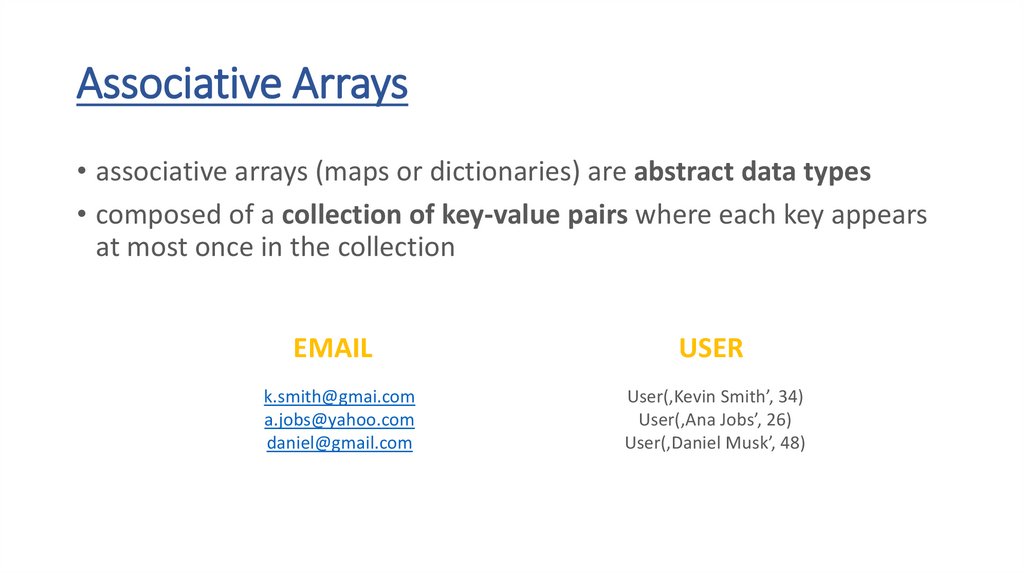
Associative Arrays• associative arrays (maps or dictionaries) are abstract data types
• composed of a collection of key-value pairs where each key appears
at most once in the collection
USER
k.smith@gmai.com
a.jobs@yahoo.com
daniel@gmail.com
User(‚Kevin Smith’, 34)
User(‚Ana Jobs’, 26)
User(‚Daniel Musk’, 48)
4.
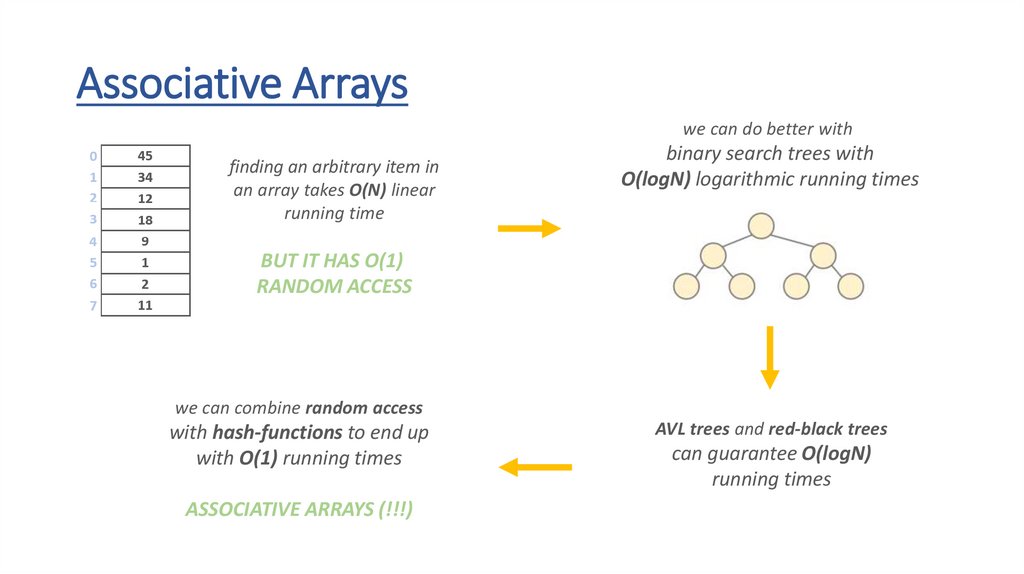
Associative Arrayswe can do better with
finding an arbitrary item in
an array takes O(N) linear
running time
binary search trees with
O(logN) logarithmic running times
BUT IT HAS O(1)
RANDOM ACCESS
we can combine random access
with hash-functions to end up
with O(1) running times
ASSOCIATIVE ARRAYS (!!!)
AVL trees and red-black trees
can guarantee O(logN)
running times
5.
Associative Arrays• there are several operations we want to implement – and we want
these operations to have O(1) running time
• adding (key, value) pairs to the collection
• removing (key, value) pairs to the collection
• lookup a given value associtaed with a given key
• The key and value pairs a– this is why associative arrays do not
support sorting as an operation
6.
Hashtables(Algorithms and Data Structures)
7.
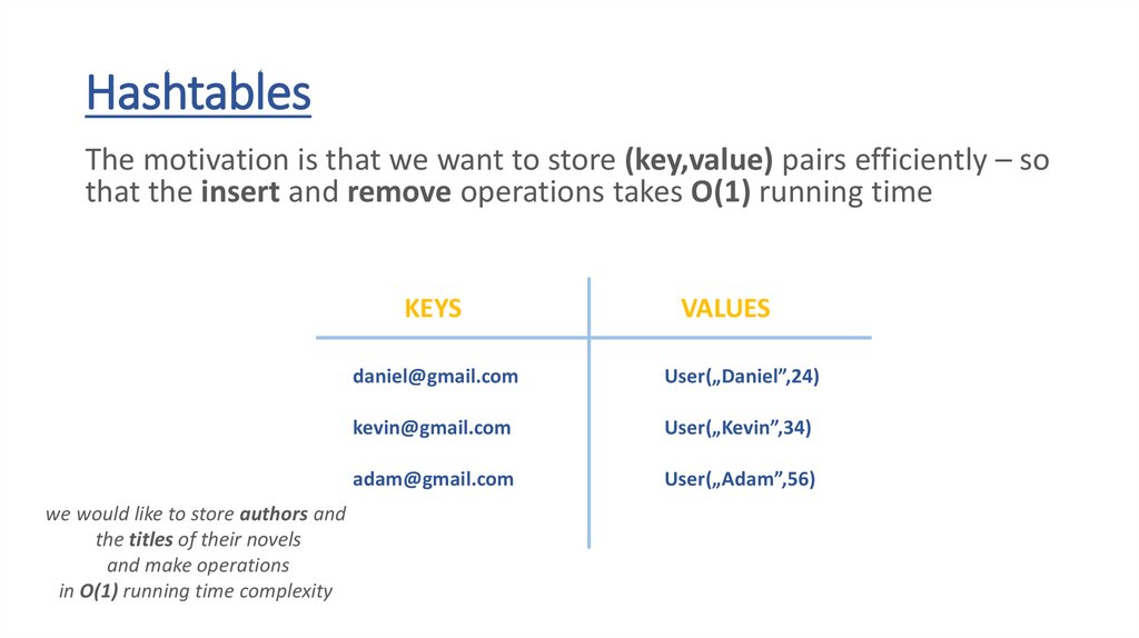
HashtablesThe motivation is that we want to store (key,value) pairs efficiently – so
that the insert and remove operations takes O(1) running time
8.
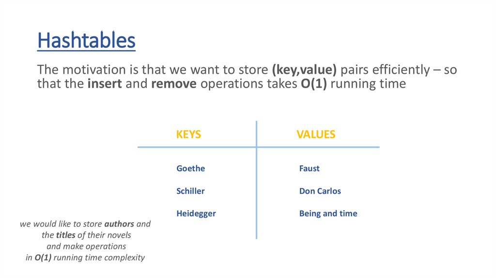
HashtablesThe motivation is that we want to store (key,value) pairs efficiently – so
that the insert and remove operations takes O(1) running time
we would like to store authors and
the titles of their novels
and make operations
in O(1) running time complexity
KEYS
VALUES
Goethe
Faust
Schiller
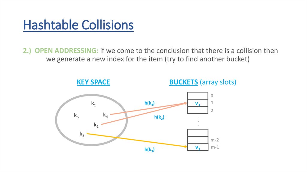
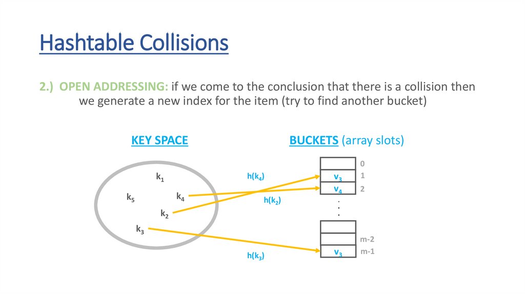
Don Carlos
Heidegger
Being and time
9.
HashtablesThe motivation is that we want to store (key,value) pairs efficiently – so
that the insert and remove operations takes O(1) running time
KEYS
we would like to store authors and
the titles of their novels
and make operations
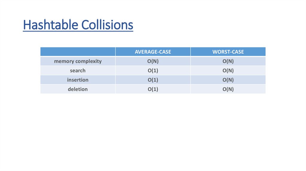
in O(1) running time complexity
VALUES
daniel@gmail.com
User(„Daniel”,24)
kevin@gmail.com
User(„Kevin”,34)
adam@gmail.com
User(„Adam”,56)
10.
HashtablesThe motivation is that we want to store (key,value) pairs efficiently – so
that the insert and remove operations takes O(1) running time
KEYS
we would like to store authors and
the titles of their novels
and make operations
in O(1) running time complexity
VALUES
daniel@gmail.com
User(„Daniel”,24)
kevin@gmail.com
User(„Kevin”,34)
adam@gmail.com
User(„Adam”,56)
11.
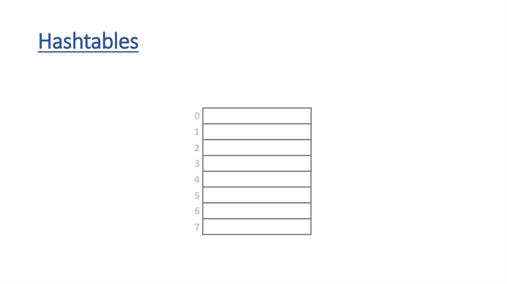
Hashtables0
1
2
3
4
5
6
7
45
34
12
18
9
1
2
11
12.
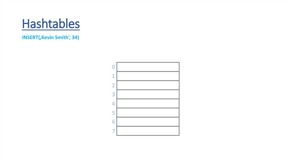
HashtablesINSERT(‚Kevin Smith’, 34)
0
1
2
3
4
5
6
7
45
34
12
18
9
1
2
11
13.
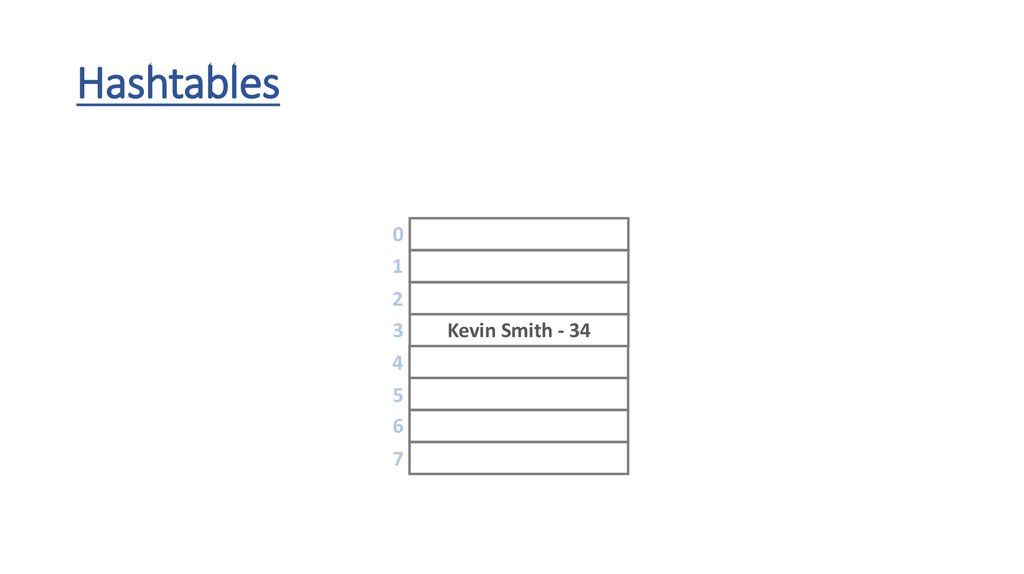
HashtablesINSERT(‚Kevin Smith’, 34)
0
1
2
3
4
5
6
7
45
34
12
Kevin Smith - 34
9
1
2
11
14.
HashtablesINSERT(‚Kevin Smith’, 34)
0
1
2
3
4
5
6
7
45
34
12
Kevin Smith - 34
9
1
2
11
15.
Hashtables0
1
2
3
4
5
6
7
45
34
12
Kevin Smith - 34
9
1
2
11
16.
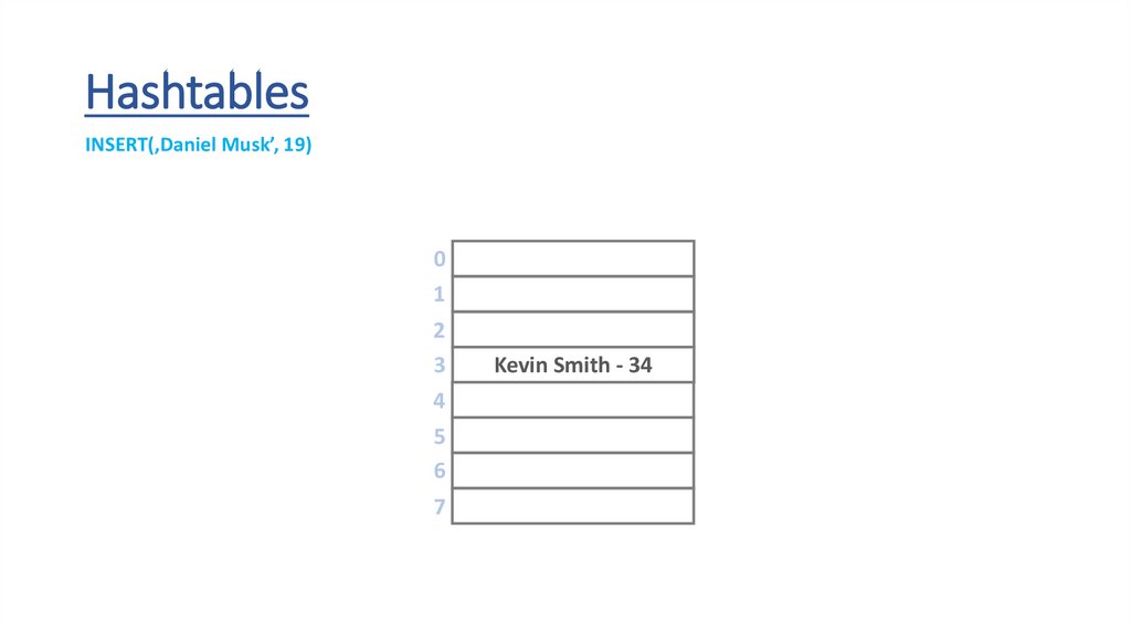
HashtablesINSERT(‚Daniel Musk’, 19)
0
1
2
3
4
5
6
7
45
34
12
Kevin Smith - 34
9
1
2
11
17.
HashtablesINSERT(‚Daniel Musk’, 19)
0
1
2
3
4
5
6
7
45
34
12
Kevin Smith - 34
9
1
Daniel Musk - 19
11
18.
Hashtables0
1
2
3
4
5
6
7
45
34
12
Kevin Smith - 34
9
1
Daniel Musk - 19
11
19.
Hashtables0
1
2
3
4
5
6
7
45
34
12
Kevin Smith - 34
9
1
Daniel Musk - 19
11
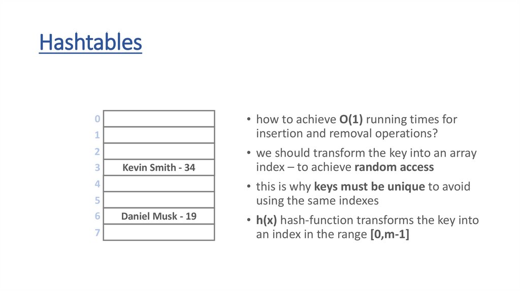
• how to achieve O(1) running times for
insertion and removal operations?
• we should transform the key into an array
index – to achieve random access
• this is why keys must be unique to avoid
using the same indexes
• h(x) hash-function transforms the key into
an index in the range [0,m-1]
20.
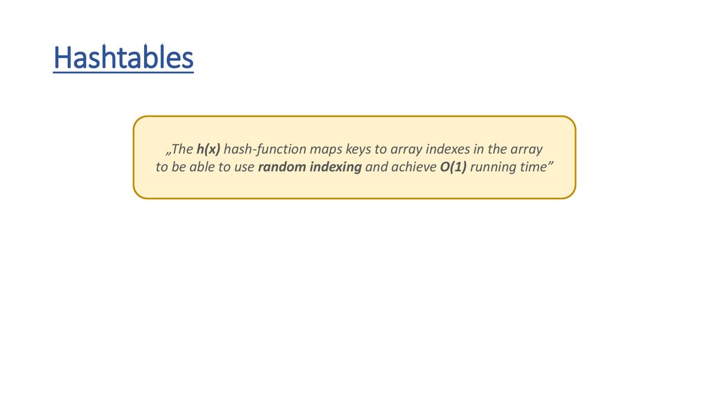
Hashtables„The h(x) hash-function maps keys to array indexes in the array
to be able to use random indexing and achieve O(1) running time”
21.
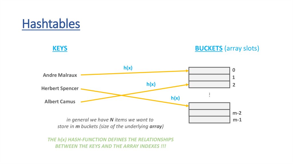
HashtablesKEYS
BUCKETS (array slots)
h(x)
0
1
2
Andre Malraux
Herbert Spencer
h(x)
Albert Camus
h(x)
in general we have N items we want to
store in m buckets (size of the underlying array)
THE h(x) HASH-FUNCTION DEFINES THE RELATIONSHIPS
BETWEEN THE KEYS AND THE ARRAY INDEXES !!!
..
.
m-2
m-1
22.
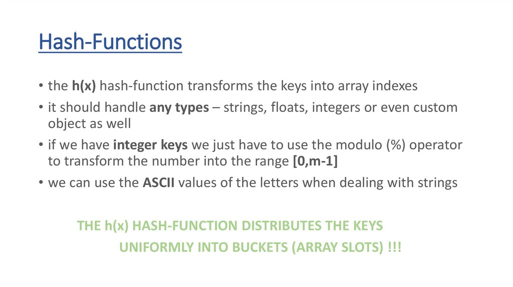
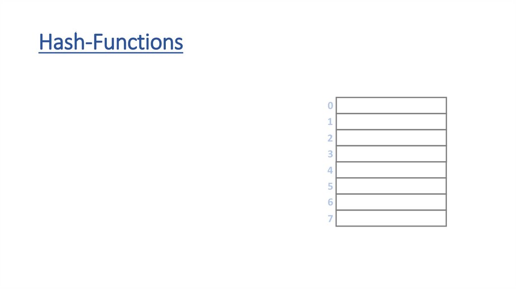
Hash-Functions• the h(x) hash-function transforms the keys into array indexes
• it should handle any types – strings, floats, integers or even custom
object as well
• if we have integer keys we just have to use the modulo (%) operator
to transform the number into the range [0,m-1]
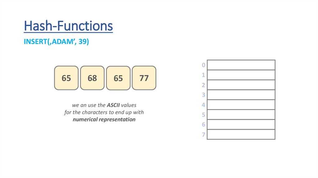
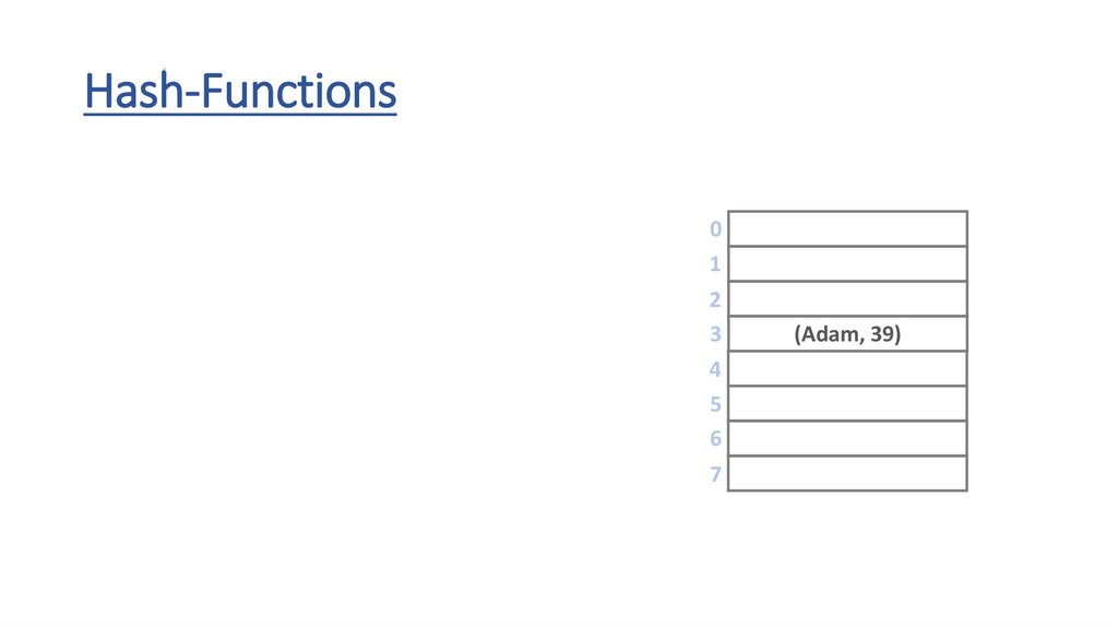
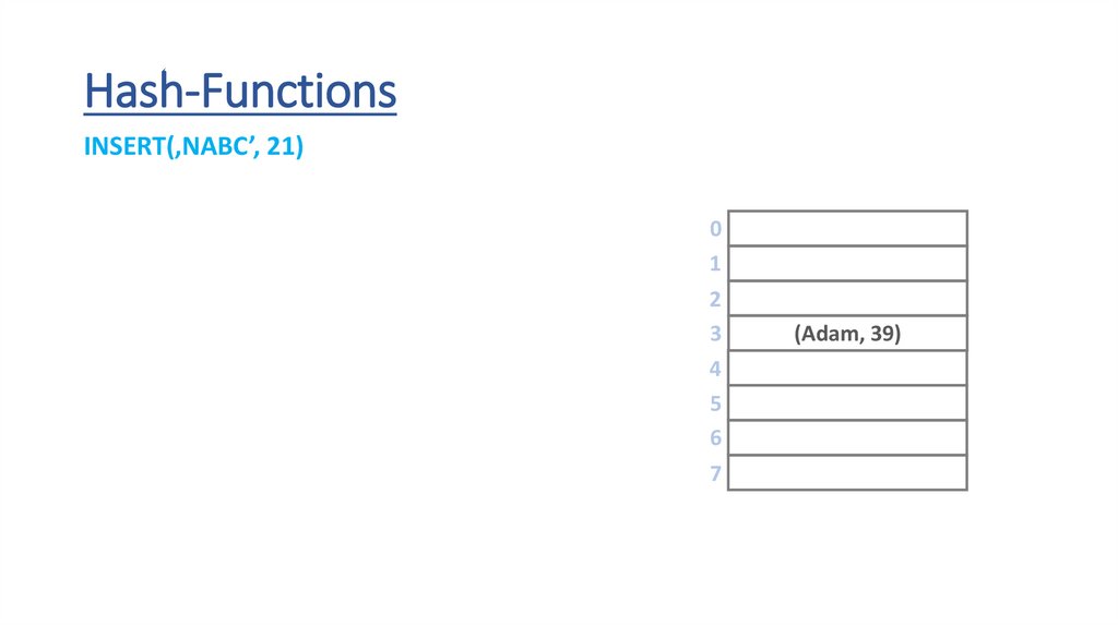
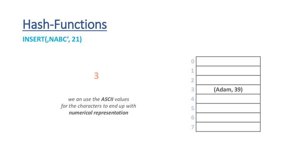
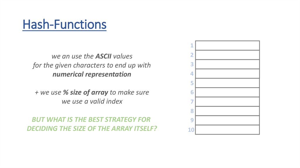
• we can use the ASCII values of the letters when dealing with strings
THE h(x) HASH-FUNCTION DISTRIBUTES THE KEYS
UNIFORMLY INTO BUCKETS (ARRAY SLOTS) !!!
23.
Hash-Functions0
1
2
3
4
5
6
7
45
34
12
18
9
1
2
11
24.
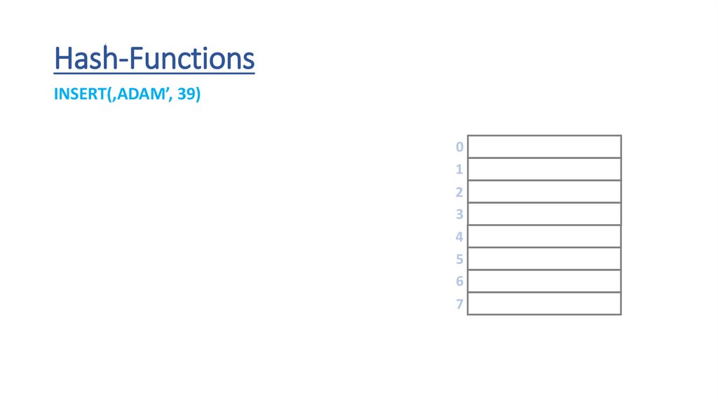
Hash-FunctionsINSERT(‚ADAM’, 39)
0
1
2
3
4
5
6
7
45
34
12
18
9
1
2
11
25.
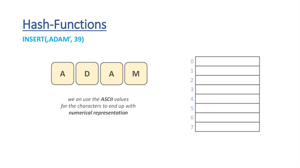
Hash-FunctionsINSERT(‚ADAM’, 39)
A
D
A
M
we an use the ASCII values
for the characters to end up with
numerical representation
0
1
2
3
4
5
6
7
45
34
12
18
9
1
2
11
26.
Hash-FunctionsINSERT(‚ADAM’, 39)
65
D
A
M
we an use the ASCII values
for the characters to end up with
numerical representation
0
1
2
3
4
5
6
7
45
34
12
18
9
1
2
11
27.
Hash-FunctionsINSERT(‚ADAM’, 39)
65
68
A
M
we an use the ASCII values
for the characters to end up with
numerical representation
0
1
2
3
4
5
6
7
45
34
12
18
9
1
2
11
28.
Hash-FunctionsINSERT(‚ADAM’, 39)
65
68
65
M
we an use the ASCII values
for the characters to end up with
numerical representation
0
1
2
3
4
5
6
7
45
34
12
18
9
1
2
11
29.
Hash-FunctionsINSERT(‚ADAM’, 39)
65
68
65
77
we an use the ASCII values
for the characters to end up with
numerical representation
0
1
2
3
4
5
6
7
45
34
12
18
9
1
2
11
30.
Hash-FunctionsINSERT(‚ADAM’, 39)
65
+
68
+
65
+
we an use the ASCII values
for the characters to end up with
numerical representation
77
0
1
2
3
4
5
6
7
45
34
12
18
9
1
2
11
31.
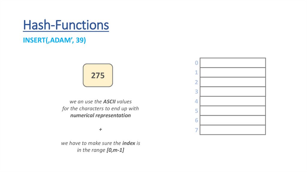
Hash-FunctionsINSERT(‚ADAM’, 39)
275
0
1
2
3
we an use the ASCII values
for the characters to end up with
numerical representation
4
5
6
+
7
we have to make sure the index is
in the range [0,m-1]
45
34
12
18
9
1
2
11
32.
Hash-FunctionsINSERT(‚ADAM’, 39)
275
%8
0
1
2
3
we an use the ASCII values
for the characters to end up with
numerical representation
4
5
6
+
7
we have to make sure the index is
in the range [0,m-1]
45
34
12
18
9
1
2
11
33.
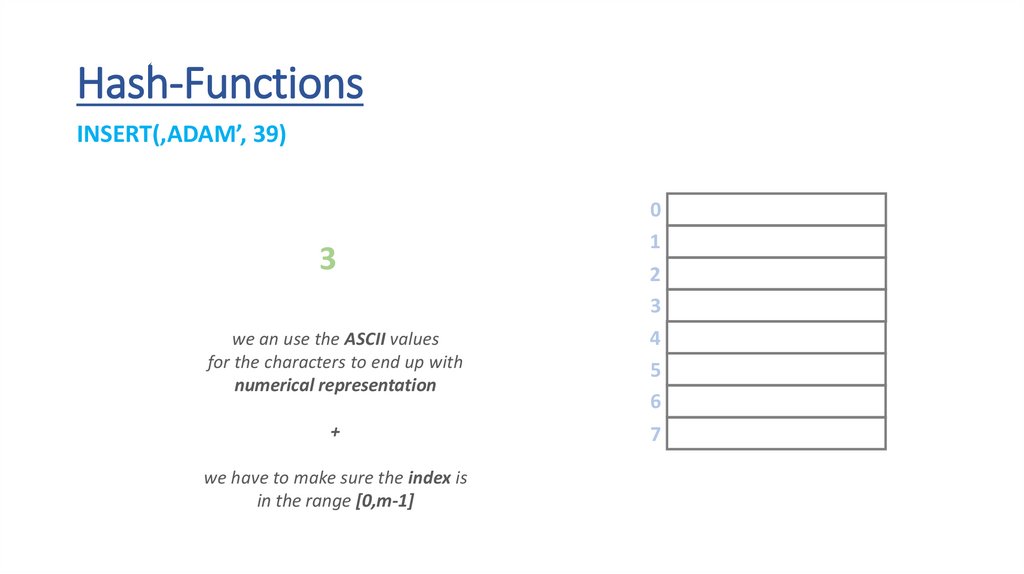
Hash-FunctionsINSERT(‚ADAM’, 39)
3
0
1
2
3
we an use the ASCII values
for the characters to end up with
numerical representation
4
5
6
+
7
we have to make sure the index is
in the range [0,m-1]
45
34
12
18
9
1
2
11
34.
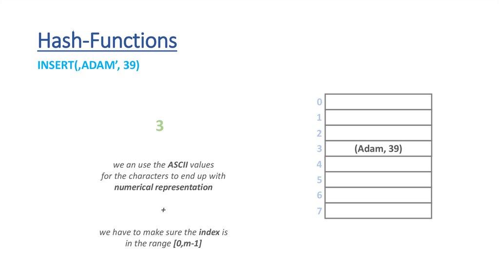
Hash-FunctionsINSERT(‚ADAM’, 39)
3
0
1
2
3
we an use the ASCII values
for the characters to end up with
numerical representation
4
5
6
+
7
we have to make sure the index is
in the range [0,m-1]
45
34
12
(Adam, 39)
9
1
2
11
35.
Hash-Functions0
1
2
3
4
5
6
7
45
34
12
(Adam, 39)
9
1
2
11
36.
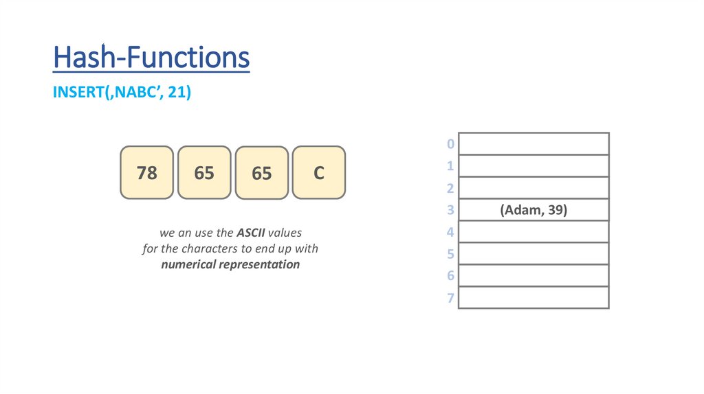
Hash-FunctionsINSERT(‚NABC’, 21)
0
1
2
3
4
5
6
7
45
34
12
(Adam, 39)
9
1
2
11
37.
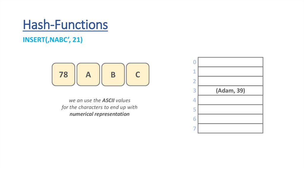
Hash-FunctionsINSERT(‚NABC’, 21)
N
A
B
C
we an use the ASCII values
for the characters to end up with
numerical representation
0
1
2
3
4
5
6
7
45
34
12
(Adam, 39)
9
1
2
11
38.
Hash-FunctionsINSERT(‚NABC’, 21)
78
A
B
C
we an use the ASCII values
for the characters to end up with
numerical representation
0
1
2
3
4
5
6
7
45
34
12
(Adam, 39)
9
1
2
11
39.
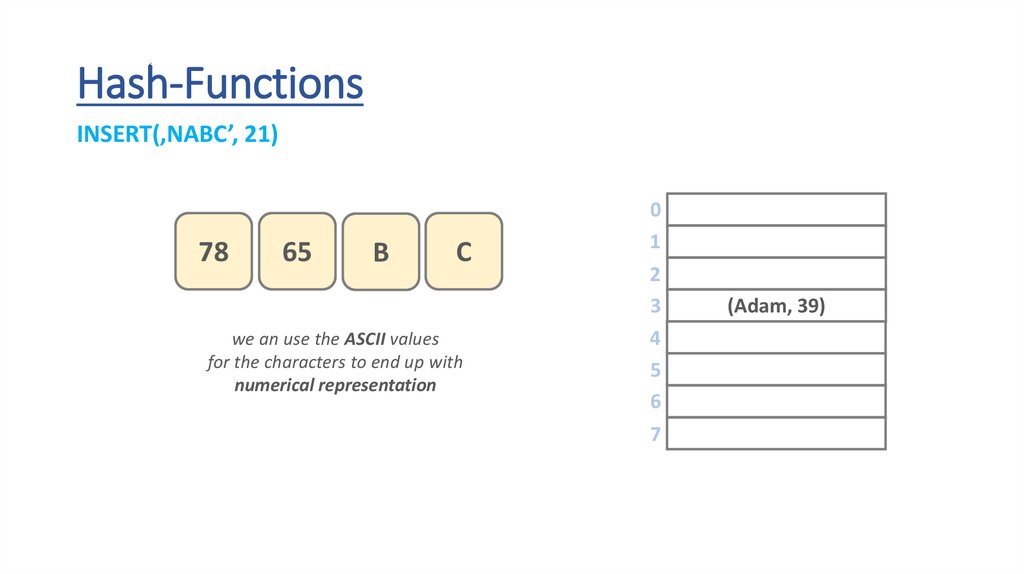
Hash-FunctionsINSERT(‚NABC’, 21)
78
65
B
C
we an use the ASCII values
for the characters to end up with
numerical representation
0
1
2
3
4
5
6
7
45
34
12
(Adam, 39)
9
1
2
11
40.
Hash-FunctionsINSERT(‚NABC’, 21)
78
65
65
C
we an use the ASCII values
for the characters to end up with
numerical representation
0
1
2
3
4
5
6
7
45
34
12
(Adam, 39)
9
1
2
11
41.
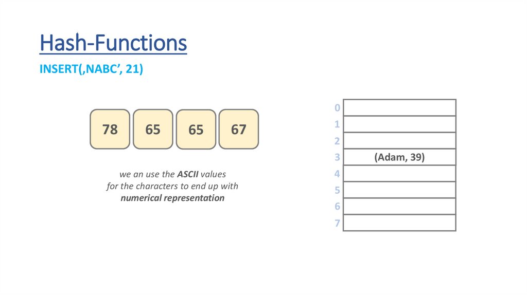
Hash-FunctionsINSERT(‚NABC’, 21)
78
65
65
67
we an use the ASCII values
for the characters to end up with
numerical representation
0
1
2
3
4
5
6
7
45
34
12
(Adam, 39)
9
1
2
11
42.
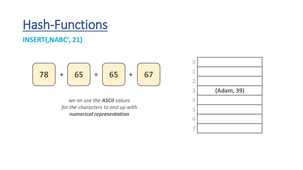
Hash-FunctionsINSERT(‚NABC’, 21)
78
+
65
+
65
+
we an use the ASCII values
for the characters to end up with
numerical representation
67
0
1
2
3
4
5
6
7
45
34
12
(Adam, 39)
9
1
2
11
43.
Hash-FunctionsINSERT(‚NABC’, 21)
275
we an use the ASCII values
for the characters to end up with
numerical representation
0
1
2
3
4
5
6
7
45
34
12
(Adam, 39)
9
1
2
11
44.
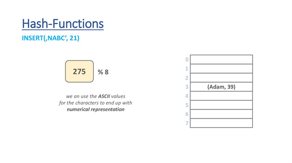
Hash-FunctionsINSERT(‚NABC’, 21)
275
%8
we an use the ASCII values
for the characters to end up with
numerical representation
0
1
2
3
4
5
6
7
45
34
12
(Adam, 39)
9
1
2
11
45.
Hash-FunctionsINSERT(‚NABC’, 21)
3
we an use the ASCII values
for the characters to end up with
numerical representation
0
1
2
3
4
5
6
7
45
34
12
(Adam, 39)
9
1
2
11
46.
Hash-FunctionsINSERT(‚NABC’, 21)
3
we an use the ASCII values
for the characters to end up with
numerical representation
0
1
2
3
4
5
6
7
45
34
12
(Adam, 39)
9
1
2
11
47.
Collisions(Algorithms and Data Structures)
48.
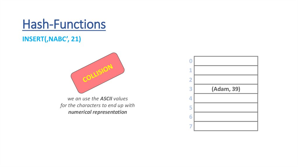
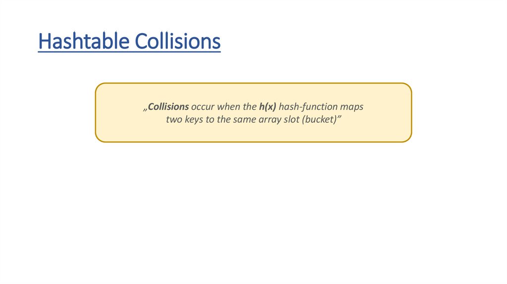
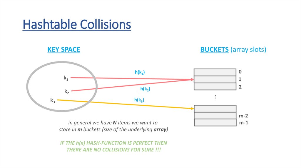
Hashtable Collisions„Collisions occur when the h(x) hash-function maps
two keys to the same array slot (bucket)”
49.
Hashtable CollisionsKEY SPACE
k1
k2
k3
BUCKETS (array slots)
0
1
2
h(k1)
h(k2)
h(k3)
in general we have N items we want to
store in m buckets (size of the underlying array)
IF THE h(x) HASH-FUNCTION IS PERFECT THEN
THERE ARE NO COLLISIONS FOR SURE !!!
..
.
m-2
m-1
50.
Hashtable Collisions• the h(x) hash-function defines the reltionships between the keys and
the array indexes (buckets)
• if the hash-function is perfect then there are no collisions
• in real-world there will be collisions becase there are no perfect
hash-functions
51.
Hashtable CollisionsThere are several approaches to deal with collisions:
1.) CHAINING
2.) OPEN ADDRESSING
52.
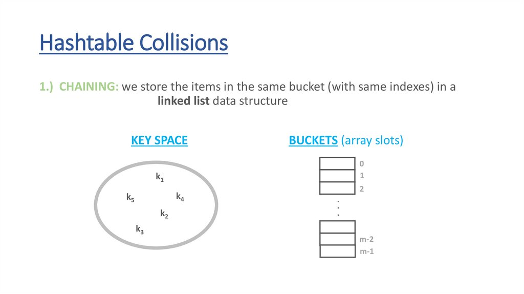
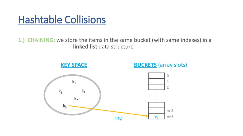
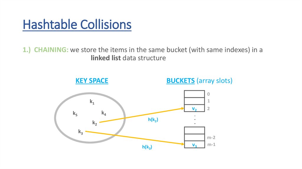
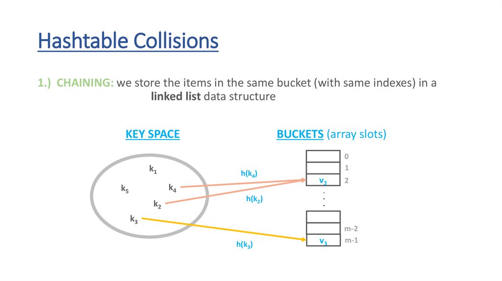
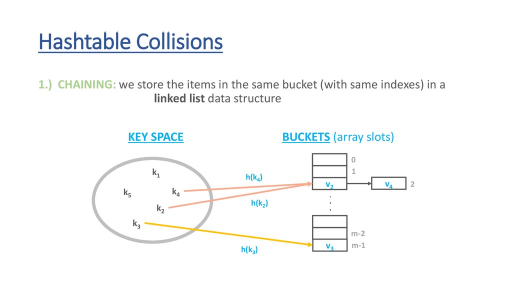
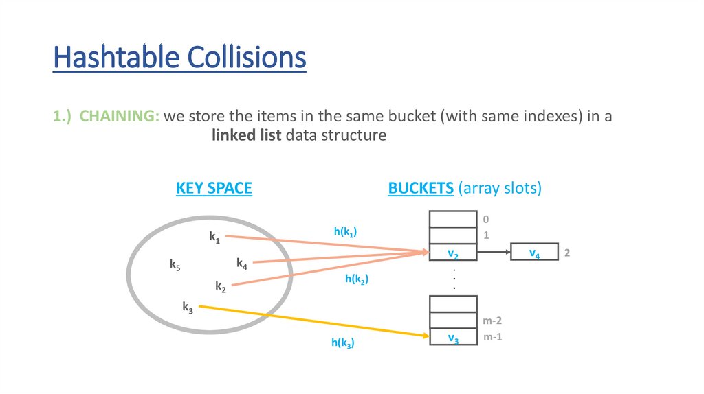
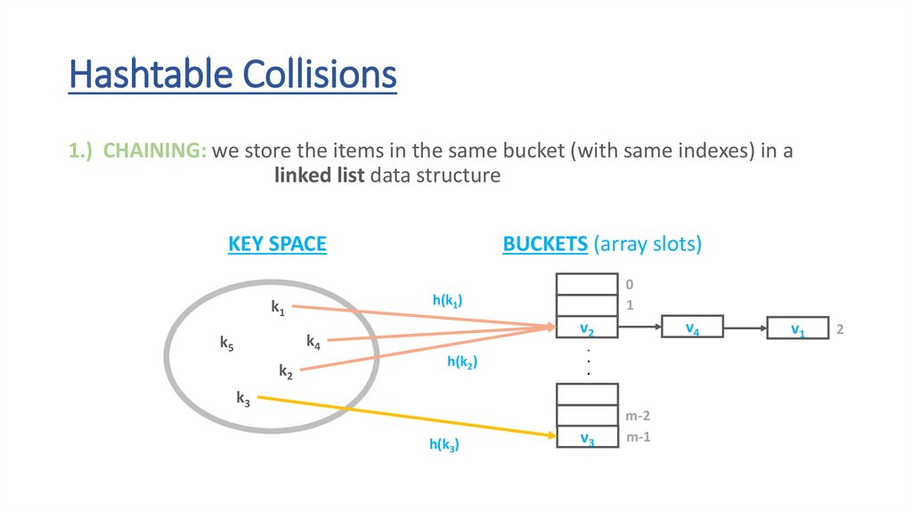
Hashtable Collisions1.) CHAINING: we store the items in the same bucket (with same indexes) in a
linked list data structure
KEY SPACE
BUCKETS (array slots)
0
1
k1
k4
k5
k2
k3
2
.
.
.
m-2
m-1
53.
Hashtable Collisions1.) CHAINING: we store the items in the same bucket (with same indexes) in a
linked list data structure
KEY SPACE
BUCKETS (array slots)
0
1
k1
2
k4
k5
.
.
.
k2
k3
h(k3)
m-2
m-1
54.
Hashtable Collisions1.) CHAINING: we store the items in the same bucket (with same indexes) in a
linked list data structure
KEY SPACE
BUCKETS (array slots)
0
1
k1
2
k4
k5
.
.
.
k2
k3
h(k3)
v3
m-2
m-1
55.
Hashtable Collisions1.) CHAINING: we store the items in the same bucket (with same indexes) in a
linked list data structure
KEY SPACE
BUCKETS (array slots)
0
1
k1
2
k4
k5
k2
h(k2)
.
.
.
k3
h(k3)
v3
m-2
m-1
56.
Hashtable Collisions1.) CHAINING: we store the items in the same bucket (with same indexes) in a
linked list data structure
KEY SPACE
BUCKETS (array slots)
0
1
k1
2
k4
k5
k2
h(k2)
.
.
.
k3
h(k3)
v3
m-2
m-1
57.
Hashtable Collisions1.) CHAINING: we store the items in the same bucket (with same indexes) in a
linked list data structure
KEY SPACE
BUCKETS (array slots)
0
1
k1
k4
k5
k2
h(k2)
v2
.
.
.
k3
h(k3)
v3
2
m-2
m-1
58.
Hashtable Collisions1.) CHAINING: we store the items in the same bucket (with same indexes) in a
linked list data structure
KEY SPACE
k1
BUCKETS (array slots)
h(k4)
k4
k5
k2
h(k2)
0
1
v2
.
.
.
k3
h(k3)
v3
2
m-2
m-1
59.
Hashtable Collisions1.) CHAINING: we store the items in the same bucket (with same indexes) in a
linked list data structure
KEY SPACE
k1
BUCKETS (array slots)
h(k4)
k4
k5
k2
h(k2)
0
1
k3
h(k3)
v4
v2
.
.
.
v3
m-2
m-1
2
60.
Hashtable Collisions1.) CHAINING: we store the items in the same bucket (with same indexes) in a
linked list data structure
KEY SPACE
BUCKETS (array slots)
h(k1)
k1
k4
k5
k2
0
1
h(k2)
k3
h(k3)
v4
v2
.
.
.
v3
m-2
m-1
2
61.
Hashtable Collisions1.) CHAINING: we store the items in the same bucket (with same indexes) in a
linked list data structure
KEY SPACE
BUCKETS (array slots)
h(k1)
k1
k4
k5
k2
0
1
h(k2)
k3
h(k3)
v4
v2
.
.
.
v3
m-2
m-1
v1
2
62.
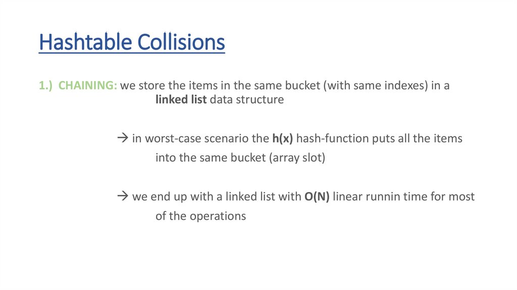
Hashtable Collisions1.) CHAINING: we store the items in the same bucket (with same indexes) in a
linked list data structure
in worst-case scenario the h(x) hash-function puts all the items
into the same bucket (array slot)
we end up with a linked list with O(N) linear runnin time for most
of the operations
63.
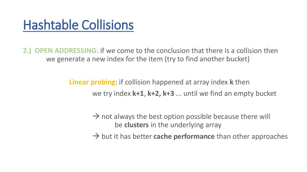
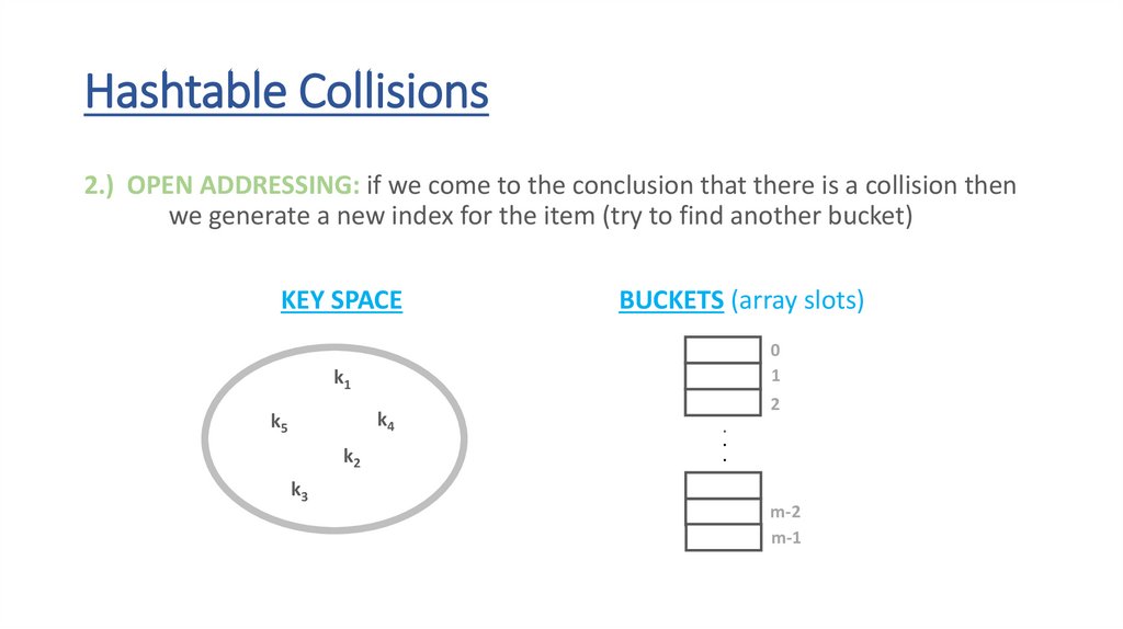
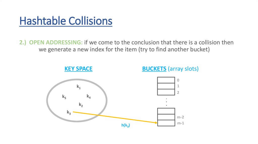
Hashtable Collisions2.) OPEN ADDRESSING: if we come to the conclusion that there is a collision then
we generate a new index for the item (try to find another bucket)
Linear probing: if collision happened at array index k then
we try index k+1, k+2, k+3 ... until we find an empty bucket
not always the best option possible because there will
be clusters in the underlying array
but it has better cache performance than other approaches
64.
Hashtable Collisions2.) OPEN ADDRESSING: if we come to the conclusion that there is a collision then
we generate a new index for the item (try to find another bucket)
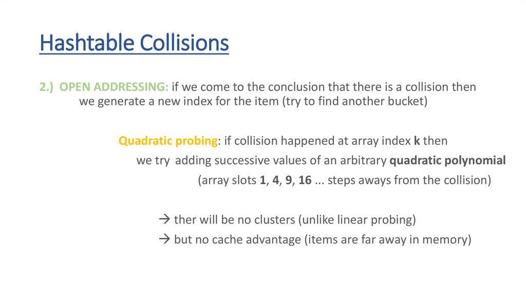
Quadratic probing: if collision happened at array index k then
we try adding successive values of an arbitrary quadratic polynomial
(array slots 1, 4, 9, 16 ... steps aways from the collision)
ther will be no clusters (unlike linear probing)
but no cache advantage (items are far away in memory)
65.
Hashtable Collisions2.) OPEN ADDRESSING: if we come to the conclusion that there is a collision then
we generate a new index for the item (try to find another bucket)
Rehasing: if collision happened at array index k then
we use the h(x) hash-function again to generate a new index
66.
Hashtable Collisions2.) OPEN ADDRESSING: if we come to the conclusion that there is a collision then
we generate a new index for the item (try to find another bucket)
KEY SPACE
BUCKETS (array slots)
0
1
k1
k4
k5
k2
k3
2
.
.
.
m-2
m-1
67.
Hashtable Collisions2.) OPEN ADDRESSING: if we come to the conclusion that there is a collision then
we generate a new index for the item (try to find another bucket)
KEY SPACE
BUCKETS (array slots)
0
1
k1
2
k4
k5
.
.
.
k2
k3
h(k3)
m-2
m-1
68.
Hashtable Collisions2.) OPEN ADDRESSING: if we come to the conclusion that there is a collision then
we generate a new index for the item (try to find another bucket)
KEY SPACE
BUCKETS (array slots)
0
1
k1
2
k4
k5
.
.
.
k2
k3
h(k3)
v3
m-2
m-1
69.
Hashtable Collisions2.) OPEN ADDRESSING: if we come to the conclusion that there is a collision then
we generate a new index for the item (try to find another bucket)
KEY SPACE
BUCKETS (array slots)
0
1
k1
k4
k5
2
h(k2)
k2
.
.
.
k3
h(k3)
v3
m-2
m-1
70.
Hashtable Collisions2.) OPEN ADDRESSING: if we come to the conclusion that there is a collision then
we generate a new index for the item (try to find another bucket)
KEY SPACE
BUCKETS (array slots)
v3
k1
k4
k5
0
1
2
h(k2)
k2
.
.
.
k3
h(k3)
v3
m-2
m-1
71.
Hashtable Collisions2.) OPEN ADDRESSING: if we come to the conclusion that there is a collision then
we generate a new index for the item (try to find another bucket)
KEY SPACE
k1
h(k4)
k4
k5
BUCKETS (array slots)
v3
0
1
2
h(k2)
k2
.
.
.
k3
h(k3)
v3
m-2
m-1
72.
Hashtable Collisions2.) OPEN ADDRESSING: if we come to the conclusion that there is a collision then
we generate a new index for the item (try to find another bucket)
KEY SPACE
k1
h(k4)
k4
k5
BUCKETS (array slots)
h(k2)
k2
v3
v4
.
.
.
k3
h(k3)
v3
0
1
2
m-2
m-1
73.
Hashtable CollisionsAVERAGE-CASE
WORST-CASE
memory complexity
O(N)
O(N)
search
O(1)
O(N)
insertion
O(1)
O(N)
deletion
O(1)
O(N)
74.
Dynamic Resizing(Algorithms and Data Structures)
75.
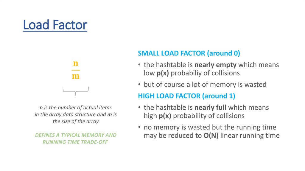
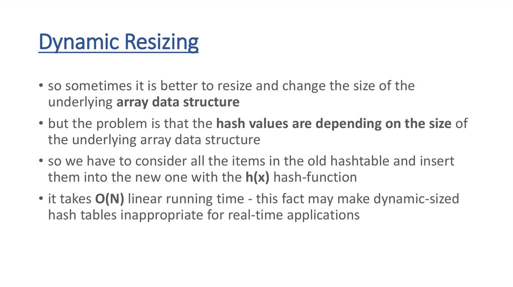
Load Factor• the p(x) probability of collision is not constant
• the more items are there in the hashtable the higher the p(x)
probability of collision
• this is why we have to define a new parameter of the hashtable – the
so-called load factor
















 Английский язык


