Environmental Modeling in Industrial Application Models for Supporting Incident Evolution: Release of Dense-than-air Pollutants

1. Environmental Modeling in Industrial Application Models for Supporting Incident Evolution: Release of Dense-than-air Pollutants

Università degli Studi di Genova
DIME
Dipartimento di Ingegneria meccanica, energetica,
gestionale e dei trasporti
Environmental Modeling in Industrial
Application
Models for Supporting Incident Evolution: Release of
Dense-than-air Pollutants
a.y. 2016-2017
Prof. Eng. Roberto Revetria PhD
Dr. Lorenzo Damiani PhD
1

2. CONTENTS

INTRODUCTION
PREVISION
MODELS
SLAB
THEORETICAL
MODEL
DESCRIPTION
ORGANIZATION
GOVERNING
EQUATIONS
TIME AVERAGED
SLAB
CONCENTRATIONS
USER GUIDE
2

3. INTRODUCTION

Emission of polluting substances can come from:
Vehicular traffic
2) Industrial plants
3) Thermo-electric plants
4) Natural sources
5) Accidents
The transport of the polluting substances in atmosphere and
their falling on the ground is a primary issue.
We need means to predict the path of the polluting cloud in
order to fulfill the required assistance and reclamation
operations.
1)
3

4. INTRODUCTION

The spatial and temporal distribution of the concentration
of the polluting substance can help to quantify:
The effects on human health (immediate or long-term
exposure)
The effects on the environment
4

5. INTRODUCTION The dense gases

The importance of the problem is very high when
dealing with:
toxic substances (SO2, Cl2 …)
flammable substances (GPL, propane, buthane …)
The gases released can be denser than air.
gases with high molecular weight
gases released in the atmosphere at low temperature
5

6. INTRODUCTION The dense gases

Example: SO2
Molecular weight (SO2) = 64 kg/kmol
Molecular weight (air) = 28.9 kg/kmol
Density:
ρ(SO2) = [M(SO2)/M(air)]* ρ(air) = 2.2 ρ(air)
6

7. Airborne chemical pollution

Attention must be paid to:
◦ accurately determine the types of pollutants taking into account
the modalities of the production process
◦ compare the reference concentrations with exposure limit
values allowed
◦ perform the technical control of concentrations, which must be
made exclusively by the source of pollution
7/24

8. Airborne chemical pollution

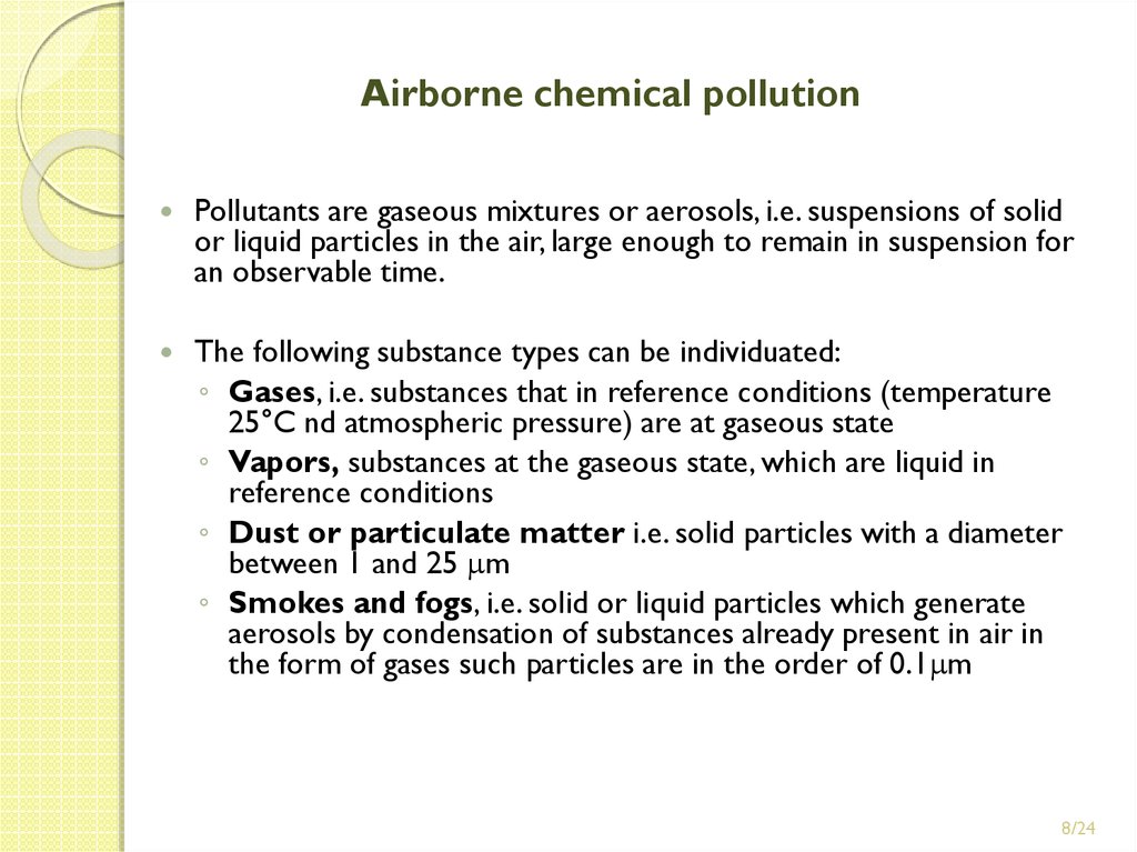
Pollutants are gaseous mixtures or aerosols, i.e. suspensions of solid
or liquid particles in the air, large enough to remain in suspension for
an observable time.
The following substance types can be individuated:
◦ Gases, i.e. substances that in reference conditions (temperature
25°C nd atmospheric pressure) are at gaseous state
◦ Vapors, substances at the gaseous state, which are liquid in
reference conditions
◦ Dust or particulate matter i.e. solid particles with a diameter
between 1 and 25 m
◦ Smokes and fogs, i.e. solid or liquid particles which generate
aerosols by condensation of substances already present in air in
the form of gases such particles are in the order of 0.1 m
8/24

9. Airborne chemical pollution

In general, toxic pollutants can penetrate in the organism through:
◦
the respiratory system
◦
the skin
◦
orally
The effects of toxic substances may consist in:
◦ forms of depression
◦ Destruction of tissues
Such effects can be:
◦ immediate
◦ protracted
◦ posticipated
The limit values are defined in relation to:
◦ Properties of the substances in the environment
◦ Results of toxicological tests
◦ epidemiological data
9/24

10. Airborne chemical pollution

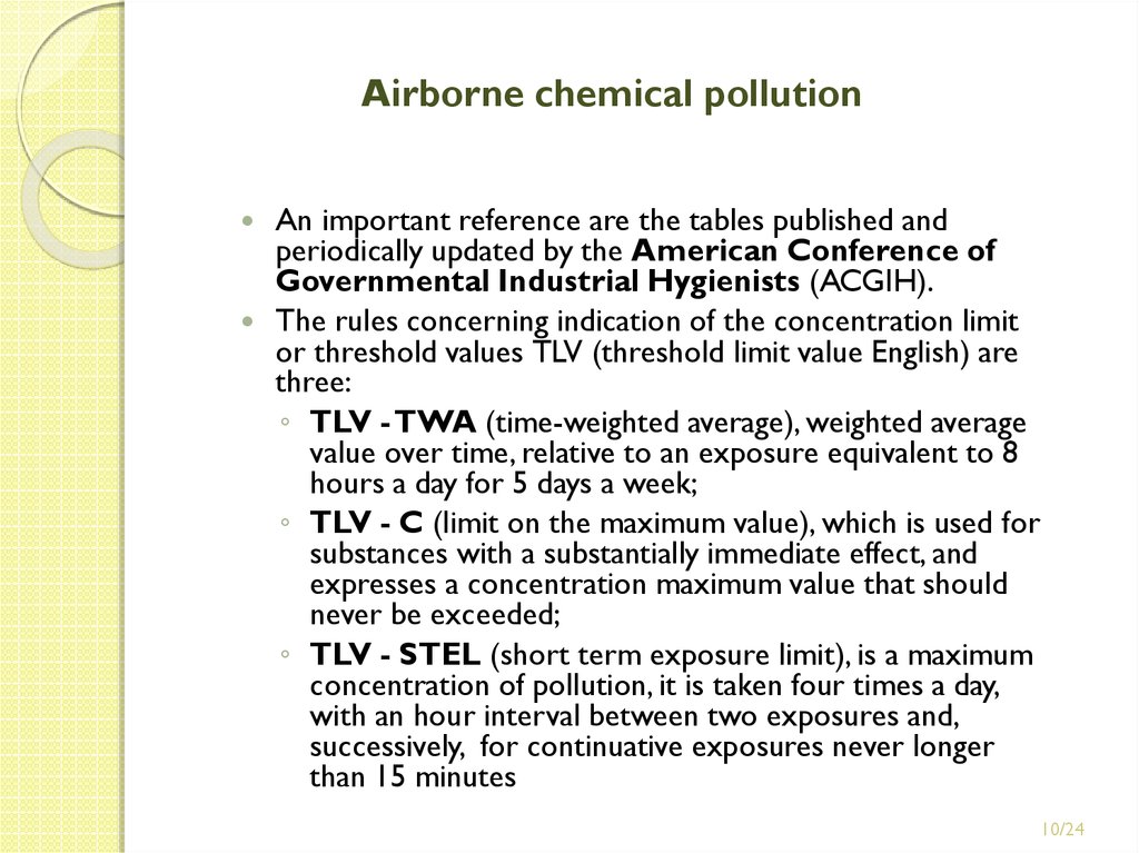
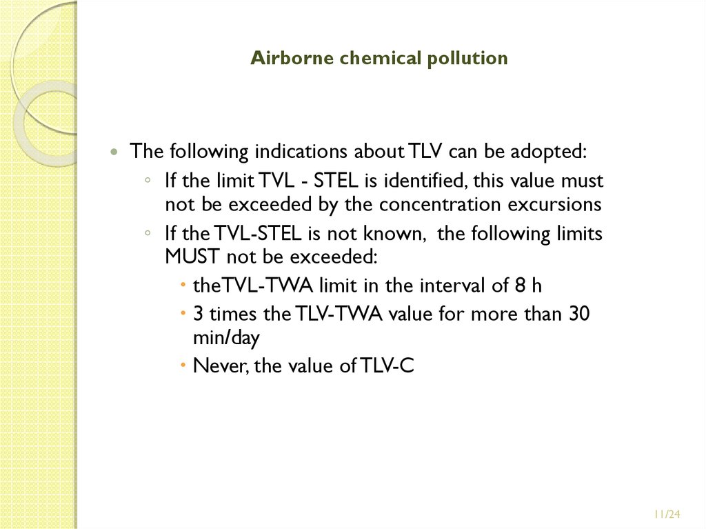
An important reference are the tables published and
periodically updated by the American Conference of
Governmental Industrial Hygienists (ACGIH).
The rules concerning indication of the concentration limit
or threshold values TLV (threshold limit value English) are
three:
◦ TLV - TWA (time-weighted average), weighted average
value over time, relative to an exposure equivalent to 8
hours a day for 5 days a week;
◦ TLV - C (limit on the maximum value), which is used for
substances with a substantially immediate effect, and
expresses a concentration maximum value that should
never be exceeded;
◦ TLV - STEL (short term exposure limit), is a maximum
concentration of pollution, it is taken four times a day,
with an hour interval between two exposures and,
successively, for continuative exposures never longer
than 15 minutes
10/24

11. Airborne chemical pollution

The following indications about TLV can be adopted:
◦ If the limit TVL - STEL is identified, this value must
not be exceeded by the concentration excursions
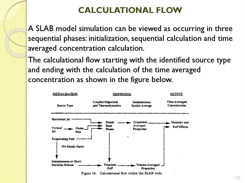
◦ If the TVL-STEL is not known, the following limits
MUST not be exceeded:
theTVL-TWA limit in the interval of 8 h
3 times the TLV-TWA value for more than 30
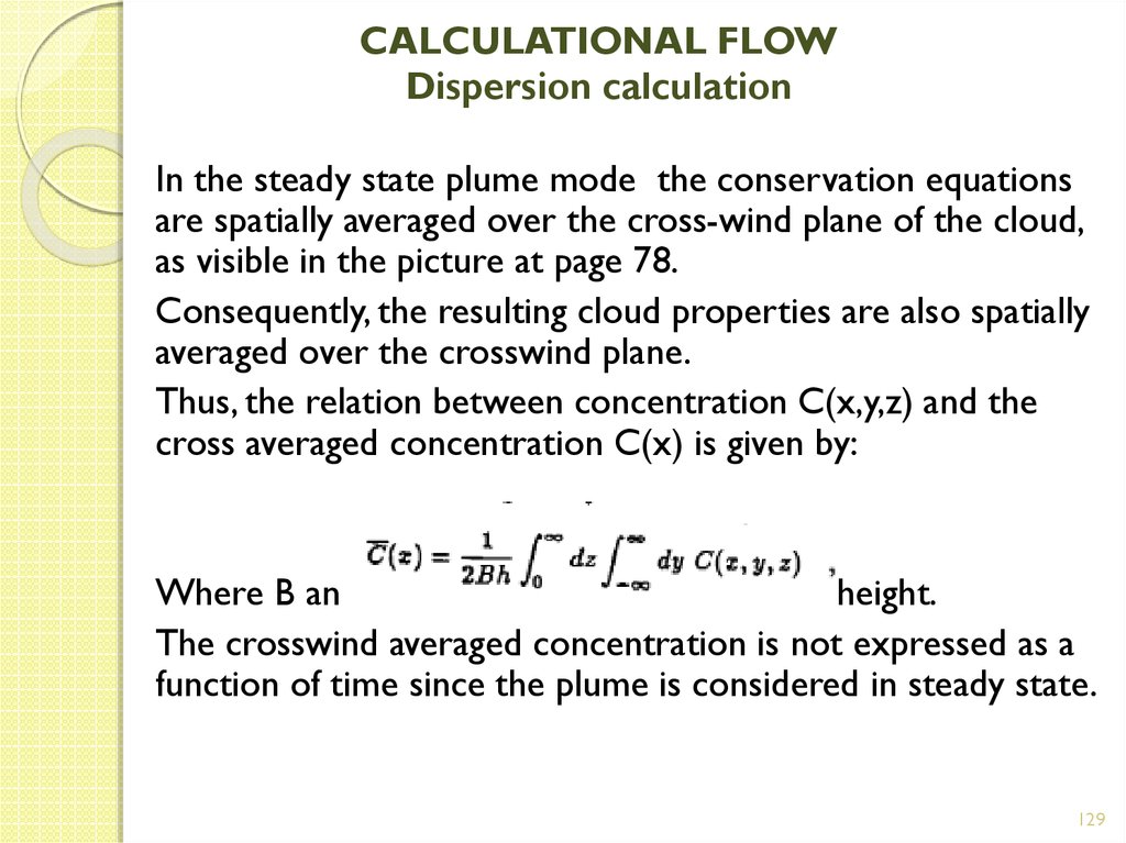
min/day
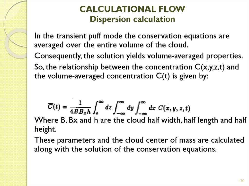
Never, the value of TLV-C
11/24

12. Airborne chemical pollution

The limits shown in the ACGIH TVL tables refer to the absorption of toxic
exclusively through the respiratory tract:
where it appears the indication "skin" beside the name of a substance, you
will have to consider the possibility of dermal absorption of the pollutant.
In case of substances with independent effect (which, i.e., produce a different
effect, or act on different parts of the body) each of them must be checked
for :
C
TLV
i
1
i
In case of substances presenting additive effect the following condition
must be verified:
C
TLV
i
i
1
i
In case of substances with singular effect, opportune deepenings are
required.
12/24

13. Airborne chemical pollution

The asphyxiating agents do not have a predetermined limit value for each
type, because:
◦ the true limiting factor is constituted by the concentration of oxygen
in the air, which should be in any case more than 18% in normal
volume at atmospheric pressure
Finally, there are some special categories of substances, on which it is
worth reflecting individually:
◦ particulates annoying but not fibrogenic (non-crystalline amorphous
silica); if the percentage of quartz is less than 1% they do not generate
serious damage
◦ fibrogenic particulates (quartz), which provoke the degeneration
of pulmonary tissues, becoming
◦ silicates (asbestos), a fundamental component of amiant;
◦ Simple asphyxiating (e.g. methane - CH4 – and carbon dioxide CO2)
◦ Variable composition substances as gasoline vapors and fumes
from welding requiring specific analyses
◦ carcinogens
13/24

14. Airborne chemical pollution

The experimental measurements for the
determination of the concentration of a pollutant in an
environment require the availability of an appropriate
instrumentation.
The analysis methodologies employed exploit
several principles:
◦ for example, it is possible to react the air volumes object of
analysis with some substances that change - in a predictable way
- the coloring (Draeger vials - a specific substance vial is
required for each type of pollutant)
14/24

15. Impact on the environment

By law, the Chemical Safety Assessment (CSA) and the
compiling of the report on chemical safety (CSR) are
mandatory for all the substances emitted in more than 10
tons/year.
All the organisms and ecosystems must be protected: the CSA
involves all these environments:
water
earth
atmosphere
predators at the vertex of the alimentary chain
micro-organisms
15/24

16. Impact on the environment

The risk evaluation for the environment based on the intrinsic
features of the substances, has the aim of:
The
evaluation for the PBT (Persistent, Bio-accumulation and
toxic) and vPvB substances
The
definition of the substance classification (e.g. dangerous
for the environment)
The
identification of the Preventable No Effect Concentration
(PNEC)
16/24

17. Impact on the environment

PBT Criteria:
Persistency
half life in sea water >60 days
half life in soft water > 40 days
half life in marine sediments > 180 days
half life in soft water sediments > 120 days
half life in the soil > 120 days
Bio-accumulation
Bio-concentration factor > 2000 – aquatic species
Toxicity
NOEC < 0.01 mg/l, aquatic organisms
Carcinogen, mutagen, toxic for reproduction
other evidences of chronic toxicity
17/24

18. Impact on the environment

vPvB Criteria:
Very persistent substance (vP)
half life in water >60 days or
half life in sediments > 180 days
half life in the soil > 180 days
Very bio-accumulable substances (vB)
Bio-concentration factor > 5000 – aquatic species
18/24

19. Impact on the environment

PNEC determination
PNEC is determined for each environmental compartment on the
basis of toxicity data for the compartment organisms (laboratory
tests)
Safety factor:
uncertainty in extrapolating the results of tests on the
environment;
high diversity of the ecosystems, experimental data only for few
species;
sensitivity of the ecosystems higher than that of the single
species.
The more numerous are the data and the analyzed species, the
lower is the safety factor.
Safety factor higher for the short-term (EC/LC50) tests than the
long-term tests.
19/24

20. Impact on the environment

Evaluation of environmental exposure
Determination of the PEC (Prevented Environmental Concentrations)
of the substance for all the compartments exposed.
• Estimation of the emissions in all the phases of the life cycle
(production, formulation, industrial use, wastes)
• Characterization of the environmental degradation, reaction,
distribution and destiny.
• PEC estimation both for regional and for local scenarios.
• PEC measured or calculated through mathematical models.
20/24

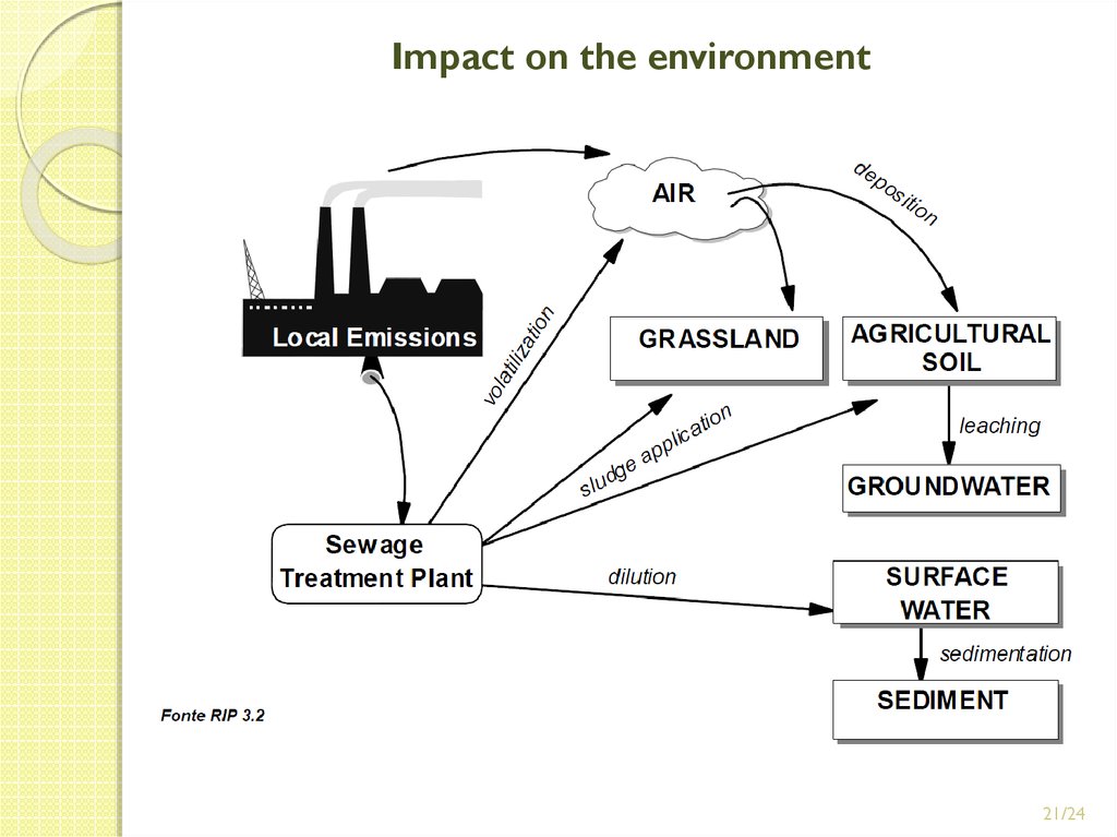
21. Impact on the environment

21/24

22. Impact on the environment

Regional PEC
Point-shaped releases diffused over a wide area have an
effect on a regional scale.
The regional PEC (stationary) provides also the
concentration in the calculation of the local PEC.
Models of regional PEC
reference area : 200X200 km2, 20 millions inhabitants,
10% production and use of the substance
The exposure models employed consist in a certain
number of homogeneous compartments (box models)
Evaluations with “multimedia fate models” based on the
concept of fugacity (e.g. Mackay).
22

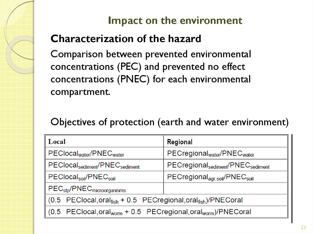
23. Impact on the environment

Characterization of the hazard
Comparison between prevented environmental
concentrations (PEC) and prevented no effect
concentrations (PNEC) for each environmental
compartment.
Objectives of protection (earth and water environment)
23

24. Impact on the environment

Characterization of the hazard
Hazards adequately controlled if PEC < PNEC.
If the condition is not satisfied, the evaluation process
can be repeated sharpening the information.
where it is not possible to determine PEC or PNEC, is
carried out a qualitative estimation of the negative effects
hazards.
If the PEC/PNEC ratio cannot be further reduced, the
substance is a candidate for measures of hazard reduction.
24

25. Phenomenology

Phenomenology of the phases of dense gases dispersion:
Source term;
Falling and gravitational slumping
Stratified dispersion
Turbulent dispersion
25

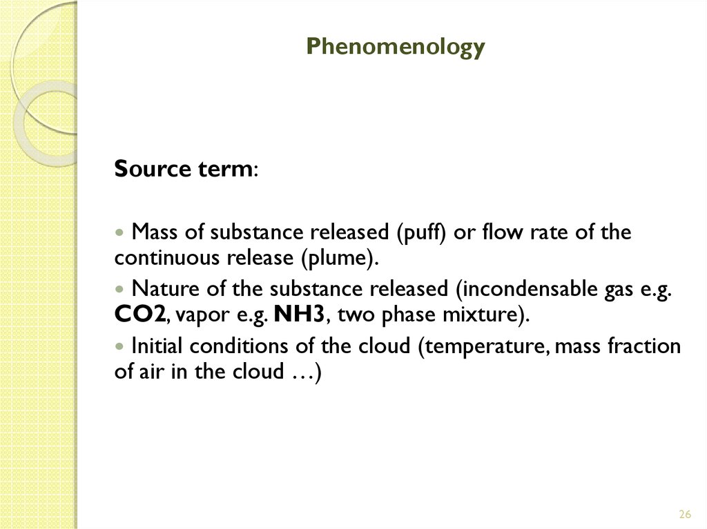
26. Phenomenology

Source term:
Mass of substance released (puff) or flow rate of the
continuous release (plume).
Nature of the substance released (incondensable gas e.g.
CO2, vapor e.g. NH3, two phase mixture).
Initial conditions of the cloud (temperature, mass fraction
of air in the cloud …)
26

27. Phenomenology

Gravitational slumping of the cloud:
The cloud formed by a denser than air release continues
to spread for the effect of gravity.
The mixing with air, particularly at the boundary on an
horizontal plane, contributes to the dilution of the
polluting cloud.
The size of the cloud continues to increase.
The gravitational slumping phase stops when the spreading
of the cloud (for gravity effect) is contrasted by the action
of the wind.
27

28. Phenomenology

Stratified dispersion:
The cloud concentration reduces further for dilution with
air, until its density becomes similar to that of air.
Turbulent dispersion:
The cloud is further dispersed in the atmosphere owing to
the turbulence of the wind flow.
28

29. PREVISION MODELS

To evaluate and quantify the dispersion of a pollutant
emission in the atmosphere, it is very useful to assume a
modelling approach.
The main types of models are:
• Stationary Gaussian models
• 3D Lagrangian models (particle models)
• 3D Eulerian models (grid models)
29

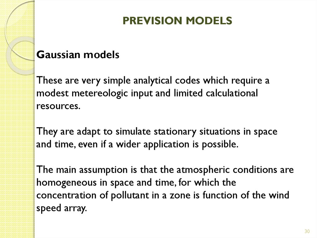
30. PREVISION MODELS

Gaussian models
These are very simple analytical codes which require a
modest metereologic input and limited calculational
resources.
They are adapt to simulate stationary situations in space
and time, even if a wider application is possible.
The main assumption is that the atmospheric conditions are
homogeneous in space and time, for which the
concentration of pollutant in a zone is function of the wind
speed array.
30

31. PREVISION MODELS

3D Lagrangian models
They simulate the dispersion of a pollutant through
computational particles displaced in the calculation domain
by the motion field and by the local turbulence conditions
of the atmosphere
3D Eulerian models
They are based on the numerical integration of balance
differential equations for each pollutant, and on the
integration of the equations representing the chemical
reactions occurring in the atmosphere.
31

32. MODELS FOR DENSE GAS RELEASES EVALUATION

Open source models
DEGADIS
SLAB
Proprietary models
AIRTOX
CHARM
FOCUS
SAFEMODE
TRACE
32

33. MODELS FOR DENSE GAS RELEASES EVALUATION

DEGADIS
DEGADIS was originally developed for the US Coast Guard
to simulate the dispersion of accidental or controlled releases
of hazardous liquids or gases in atmosphere.
DEGADIS includes a module for predicting the trajectory and
dilution of an elevated dense gas jet.
The concentration/density relation is described using ordered
triplets consisting of mole fraction, concentration and mixture
density.
DEGADIS contains an internal chemical library that provides
the properties of the chemical to be modeled
33

34. MODELS FOR DENSE GAS RELEASES EVALUATION

SLAB
SLAB was developed by Lawrence Livermore National Lab to
simulate the release of denser than air gases.
SLAB models 4 categories of releases: evaporating pools,
vertical jets, horizontal jets and instantaneous releases.
Releases can be treated as transient or steady state, or a
combination of both.
SLAB does not contain an internal chemical library, but the
user’s guide provides the parameters for many substances of
interest.
34

35. MODELS FOR DENSE GAS RELEASES EVALUATION

AIRTOX
AIRTOX has been developed by ENSR Consulting and
Engineering to calculate downwind concentrations from time
dependent toxic releases to the atmosphere
Chemical releases are simulated either in jet or in non-jet
mode.
AIRTOX is a spreadsheet based model, that utilizes Lotus 123
software.
Chemical properties are provided through the internal
database.
35

36. MODELS FOR DENSE GAS RELEASES EVALUATION

CHARM
CHARM is a Gaussian puff model created by Radian
Corporation to assess the location, extent and concentration
of the cloud resulting from the release of a toxic substance.
CHARM includes a chemical database that provides all the
necessary chemical parameters of the model.
CHARM is a menu driven system composed of 2 parts: one
containing all the screens for data input, the other one
performing the calculations.
Model results are provided in a graphical display, providing a
snapshot of the cloud passage with time.
36

37. MODELS FOR DENSE GAS RELEASES EVALUATION

FOCUS
MODELS FOR DENSE GAS RELEASES
EVALUATION
FOCUS is a hazards analysis software package designed by
Quest Consultants Inc. to evaluate transient hazards resulting
from accidental or controlled releases of liquids and gases.
FOCUS predicts hazard zones resulting from fires and
explosions, and vapor clouds formed from release of toxic
and/or flammable materials.
The model provides downwind centerline concentrations as a
function of time since release and the lateral distance to three
user- specified concentration limits.
The predicted concentrations represent values averaged over
the release duration.
37

38. MODELS FOR DENSE GAS RELEASES EVALUATION

SAFEMODE
SAFEMODE was developed by Technology and Management
Systems Inc.
It is a tool for assessing the potential for acute hazards arising
from the accidental release of toxic chemicals.
The user specifies source/release conditions in detail,
including container dimensions, chemical name, storage
condition, leak geometry and environmental conditions.
Predicted concentrations are displayed graphically as
contours.
SAFEMODE has an internal database of more than 100
substances.
38

39. MODELS FOR DENSE GAS RELEASES EVALUATION

TRACE
TRACE was developed by EI Dupont De Nemours Company.
TRACE is an interactive menu driven model that allows the
user multiple options when developing a release scenario. It
contains an extensive chemical library.
The TRACE model output provides information about vapor
cloud dynamics, snapshots of concentration isophlets and
receptor impacts.
The cloud dynamics section displays various cloud parameters
as a function of time after release.
39

40. SLAB

40

41. INTRODUCTION

SLAB is a computer code that simulates the atmospheric
dispersion of denser than air releases.
The last version of SLAB can treat continuous, finite duration
and instantaneous release from 4 types of source:
A ground level evaporating pool,
An elevated horizontal jet
A stack (elevated vertical jet)
A ground based instantaneous release.
The evaporating pool source is assumed to be pure vapor, in
accordance with the evaporation process
The other sources can be either pure vapor or a mixture of vapor
and liquid
41

42. INTRODUCTION

Atmospheric dispersion of the release is calculated by
solving the conservation equations of
Mass
Momentum
Energy
Species
To simplify the solution of the conservation equations, the
equations are spatially averaged with the cloud.
42

43. INTRODUCTION

The cloud can be modeled as a steady-state plume or
as a puff, as visible in Figures 1 and 2.
43

44. INTRODUCTION

A continuous release (very long emission duration) is treated as
a plume.
In the case of a finite duration release, cloud dispersion is
initially described using the steady state plume mode, and
remains in this mode as long as the source is active.
Once the source is shut off, the cloud is treated as a transient
puff and the subsequent dispersion is calculated using the puff
mode.
For an instantaneous release (explosion), the transient puff
dispersion mode is used for the entire calculation.
44

45. INTRODUCTION

Solution of the spatially-averaged conservation equations
in either dispersion mode yields the spatially-averaged
cloud properties.
To regain the 3D variation of the concentration
distribution, are applied particular profile functions of an
assumed form and dependence on the calculated cloud
dimensions.
45

46. INTRODUCTION

The time averaged concentration is obtained in a two step
process:
1) The effect of the cloud meander on the effective width of
the cloud is calculated;
2) The concentration is averaged over time using the
effective (meander included) width in the concentration
profile function.
This calculation yields the final results of the SLAB model,
namely, the time averaged concentration in time and space.
46

47. MODEL ORGANIZATION

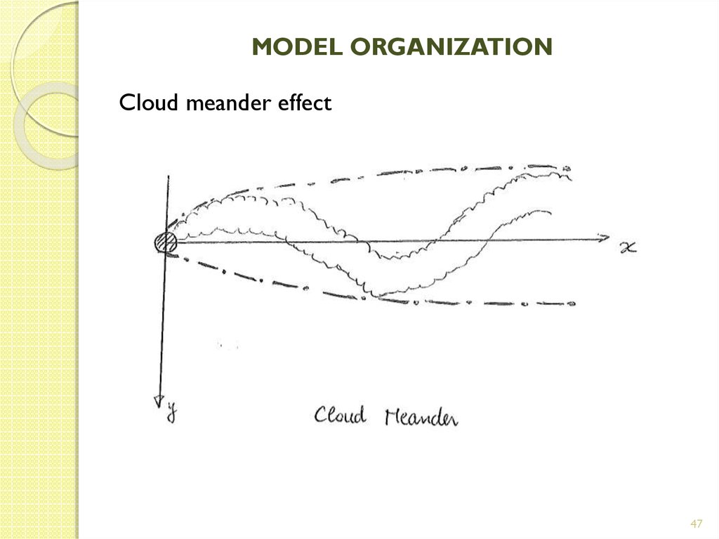
Cloud meander effect
47

48. THEORETICAL DESCRIPTION

The atmospheric dispersion of a large denser than air release is
affected by phenomena that do not occur in neutrally or
positively buoyant trace gas releases:
Turbulence damping due to stable density stratification of the
heavy gas cloud;
Alteration of the ambient velocity field due to gravity flow and
initial source momentum;
Thermodynamic effects on cloud temperature, buoyancy and
turbulence due to liquid droplet formation and evaporation, and
ground heating in the case of the release of a superheated or
cryogenic liquid
48

49. THEORETICAL DESCRIPTION

In combustible gas releases one can be concerned with the
instantaneous concentration.
In toxic gas releases, the concern can be about doses over
minutes or hours as well as the long term dose.
In order to make meaningful predictions of the size and
duration of the hazardous concentration from a dense gas
release, all of the significant phenomena need to be
included, and the appropriate concentration averaging time
needs to be used.
49

50. THEORETICAL DESCRIPTION

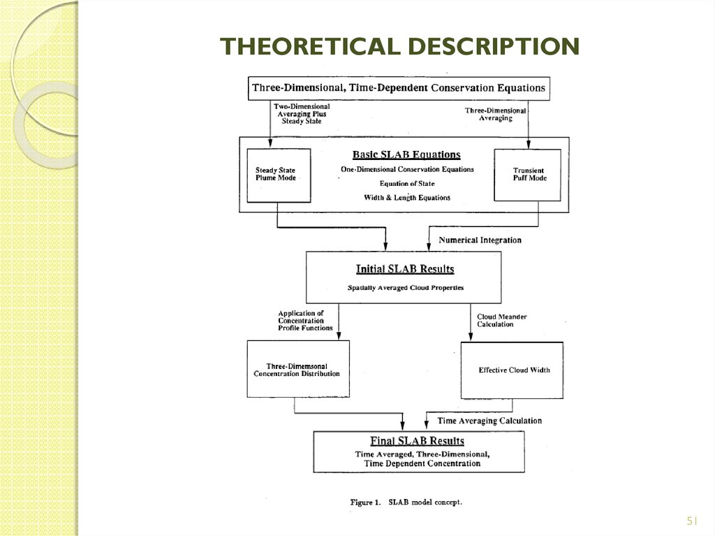
To meet these requirements, the SLAB model is built upon
a theoretical framework that starts with averaged forms of
the conservation equations of mass, momentum, energy
and species (see figure in the next page).
These equations are used to calculate the spatially-averaged
properties of the dispersing cloud and are expressed in
two forms, representing two different dispersion modes:
1) Steady state plume
2) Transient puff.
50

51. THEORETICAL DESCRIPTION

51

52. THEORETICAL DESCRIPTION

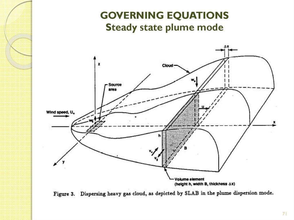
The conservation equations are different for the two
modes, plume and puff.
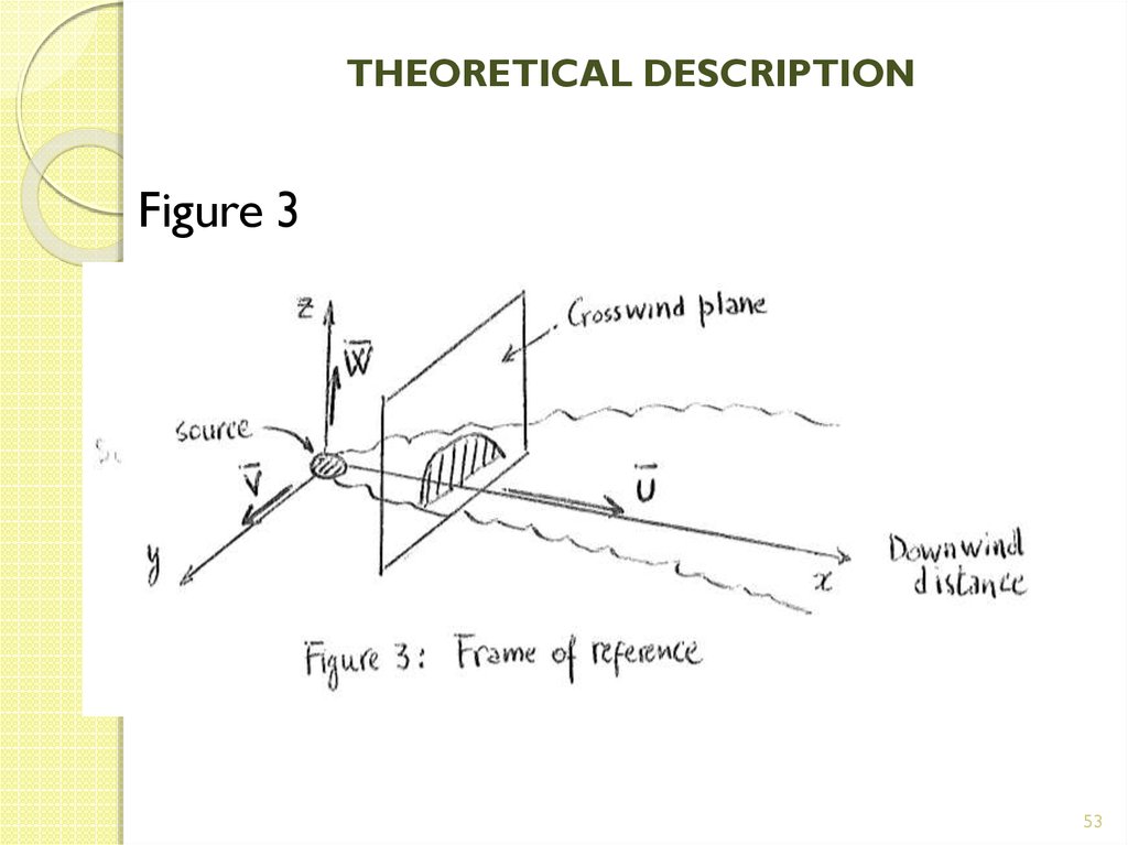
The steady state plume form of the equations is obtained
by making the steady state assumption (d/dt =0) and by
averaging the equations over the cross wind direction (y
and z, see figure 3 next page).
The transient puff form of the equations is obtained by
averaging the equations over all the three directions (x, y,
z).
52

53. THEORETICAL DESCRIPTION

Figure 3
53

54. THEORETICAL DESCRIPTION

The theoretical framework of the SLAB model is
completed by the inclusion of the equation of state
(ideal gas law) and equations of the growth of cloud
dimensions (plume width in the steady state mode and
puff length and width in the transient puff mode)
54

55. THEORETICAL DESCRIPTION

To solve the basic set of equations, additional submodels
are required.
These submodels describe the dilution of the cloud due to
The turbulent mixing with surrounding air,
the formation and evaporation of liquid droplets within
the cloud and
the heating of cold clouds at the ground surface.
55

56. THEORETICAL DESCRIPTION

The turbulent mixing with surrounding air, is treated by
using the entrainment concept which specifies the rate of
air flow into the cloud.
The thermodynamics of liquid droplets within the cloud is
modeled by using the local thermodynamic equilibrium
approximation.
The size of the liquid droplets is assumed to be sufficiently
small so that the transport of the vapor-droplet mixture
can be treated as a single fluid.
Ground heating of the cloud is treated by using the
radiation boundary condition and a coefficient of surface
and heat transfer.
56

57. THEORETICAL DESCRIPTION

In the steady state plume mode the conservation
equations are averaged over the cross wind plan of the
plume, leaving the downwind distance (x) as the single
independent variable.
In the transient puff mode the conservation equations are
averaged over all three dimensions of the cloud, leaving the
downwind travel time (t) of the puff as a single
independent variable.
Notice that travel time (t) and downwind distance (x) are
related by the downwind cloud velocity (U)
57

58. THEORETICAL DESCRIPTION

The 3D concentration distribution of the cloud is
determined from the average concentration and by using
similarity profiles that include the calculated cloud
dimensions.
Thus, the code is 1D in both puff and plume modes, but can
be seen as quasi 3D, as the cloud dimensions are used to
specify the spatial distribution of the cloud.
For most code users, the most important result is the time
averaged volume concentration in function of travel time
(t), from the source, and as a function of the three spatial
dimensions.
58

59. MODEL ORGANIZATION

The calculational flow within the SLAB code is reported in
Figure below
59

60. MODEL ORGANIZATION

There are three stages in a typical simulation:
Source identification and initialization for dispersion;
2) Calculation of cloud dispersion;
3) Calculation of the time-averaged concentration
1)
The choice between plume or puff mode depends on the
type of source and the duration of the spill.
60

61. MODEL ORGANIZATION

Dispersion from an evaporating pool and a horizontal jet both
begin in the steady state plume mode.
This mode has two regions:
1) A source region where source material is added to the
dispersing cloud.
2) A near-field region, where no additional source material is
added to the cloud but it is still in steady state.
The calculation of evaporating pool begins in the source region and
proceeds to the near field region.
The horizontal jet source begins with a pure source emission
cloud travelling downwind at a speed equal to the jet exit velocity.
61

62. MODEL ORGANIZATION

The situation for the vertical jet is similar to that of
the horizontal jet; however, the vertical jet has a plume rise
region where the cloud motion is mainly vertical.
Consequently, the plume rise calculation is completed before
entering the steady state near field plume dispersion
calculation.
62

63. MODEL ORGANIZATION

The dispersion calculation for a continuous but limited release of
duration t_sd is initially conducted in the steady state plume mode.
In this mode, the downwind distance x is the independent variable
and time t is taken to be proportional to the amount of emitted
mass within the plume.
Calculation of the plume properties in function of x continues until
the emitted mass within the plume, from the upwind edge of the
cloud to the downwind distance Xt, is equal to one half of the
released mass Qs.
At this downwind location, the dispersion calculation is switched
from the plume mode to the puff mode.
63

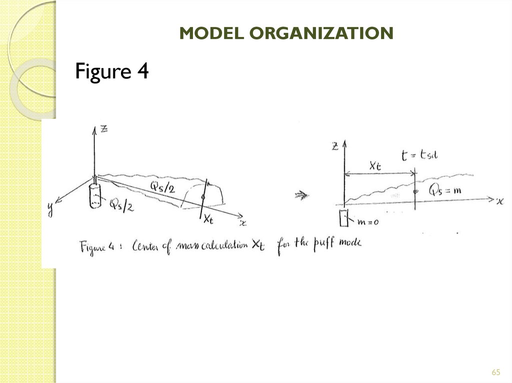
64. MODEL ORGANIZATION

The puff center of mass is set equal to Xt, so that the
emitted mass within the puff is equal to the total mass
released Qs, with half the mass upwind of Xt and half the
mass downwind (see figure 4)
Time t is the single independent variable in the puff mode,
and the time of transition from the plume to the puff mode is
taken to occur at the end of the release when t = t_sd.
64

65. MODEL ORGANIZATION

Figure 4
65

66. MODEL ORGANIZATION

An exception to this procedure is taken when an
evaporating pool release fails to reach steady state within the
source region. (short duration evaporating pool)
This occurs whenever the emitted mass within the source
region of the steady state plume is greater than the total
released mass Qs.
When this occurs, the steady state calculation is discarded
and the entire calculation is restarted in the transient puff
mode.
In case of instantaneous source there is also no steady state
cloud.
66

67. MODEL ORGANIZATION

Completion of the dispersion calculations in either mode,
yields the instantaneous spatially averaged cloud properties:
mass and volume concentration, density, temperature,
downwind velocity, cloud dimensions etc.
The 3D variation of the concentration distribution is
accounted for by applying profile functions that are based on
the calculated cloud dimensions.
67

68. MODEL ORGANIZATION

The calculation of the time-averaged concentration is conducted
in 2 steps:
The effective cloud width, which includes the increase due to
cloud meander, is determined. (N.B.: instantaneous cloud width
does not include the effect of cloud meander, which is the nonstationary displacement in the cross-wind direction). The
amount of increase in width depends on the duration of
averaging time, the duration of release and the instantaneous
cloud width
2) The time averaged concentration is calculated from the “new”
concentration distribution, which includes the effect of cloud
meander in the effective cloud width.
1)
68

69. MODEL ORGANIZATION

Cloud meander effect
69

70. GOVERNING EQUATIONS Steady state plume mode

The steady state plume mode of SLAB is based on the
steady state crosswind-averaged conservation equations of
mass, momentum, energy and species,
It uses the air entrainment concept to account for turbulent
mixing of the gas cloud with the surrounding atmosphere, as
shown in the figure in the following page.
70

71. GOVERNING EQUATIONS Steady state plume mode

71

72. GOVERNING EQUATIONS Steady state plume mode

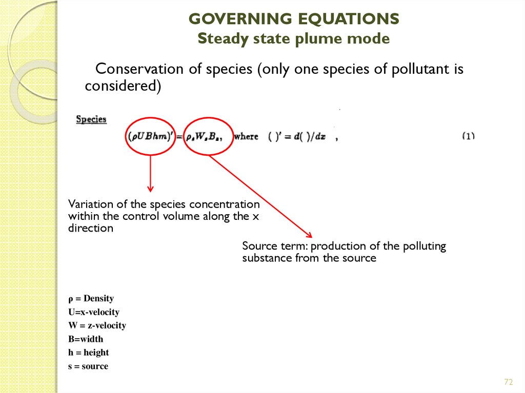
Conservation of species (only one species of pollutant is
considered)
Variation of the species concentration
within the control volume along the x
direction
Source term: production of the polluting
substance from the source
ρ = Density
U=x-velocity
W = z-velocity
B=width
h = height
s = source
72

73. GOVERNING EQUATIONS Steady state plume mode

Conservation of mass
Variation in the x
direction of the mass
contained within the
control volume
Source term: production of the polluting
substance from the source
Flow term: air mass flow through the
walls of the control volume
ρ = Density
U=x-velocity
V = y-velocity, W= z-velocity
B=width
h = height
s = source , e= external
73

74. GOVERNING EQUATIONS Steady state plume mode

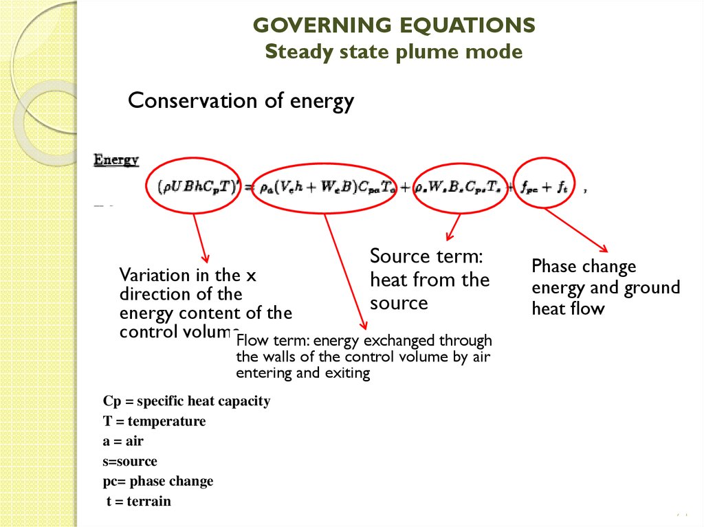
Conservation of energy
Source term:
heat from the
source
Variation in the x
direction of the
energy content of the
control volumeFlow term: energy exchanged through
Phase change
energy and ground
heat flow
the walls of the control volume by air
entering and exiting
Cp = specific heat capacity
T = temperature
a = air
s=source
pc= phase change
t = terrain
74

75. GOVERNING EQUATIONS Steady state plume mode

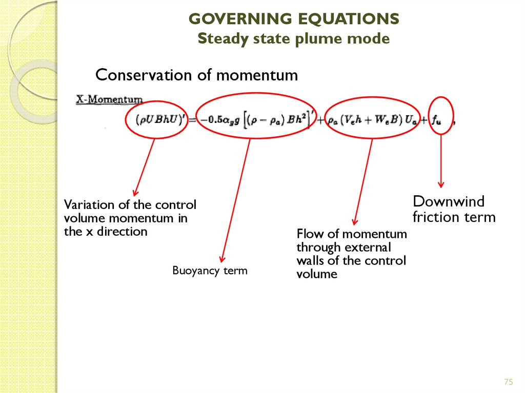
Conservation of momentum
Variation of the control
volume momentum in
the x direction
Buoyancy term
Flow of momentum
through external
walls of the control
volume
Downwind
friction term
75

76. GOVERNING EQUATIONS Steady state plume mode

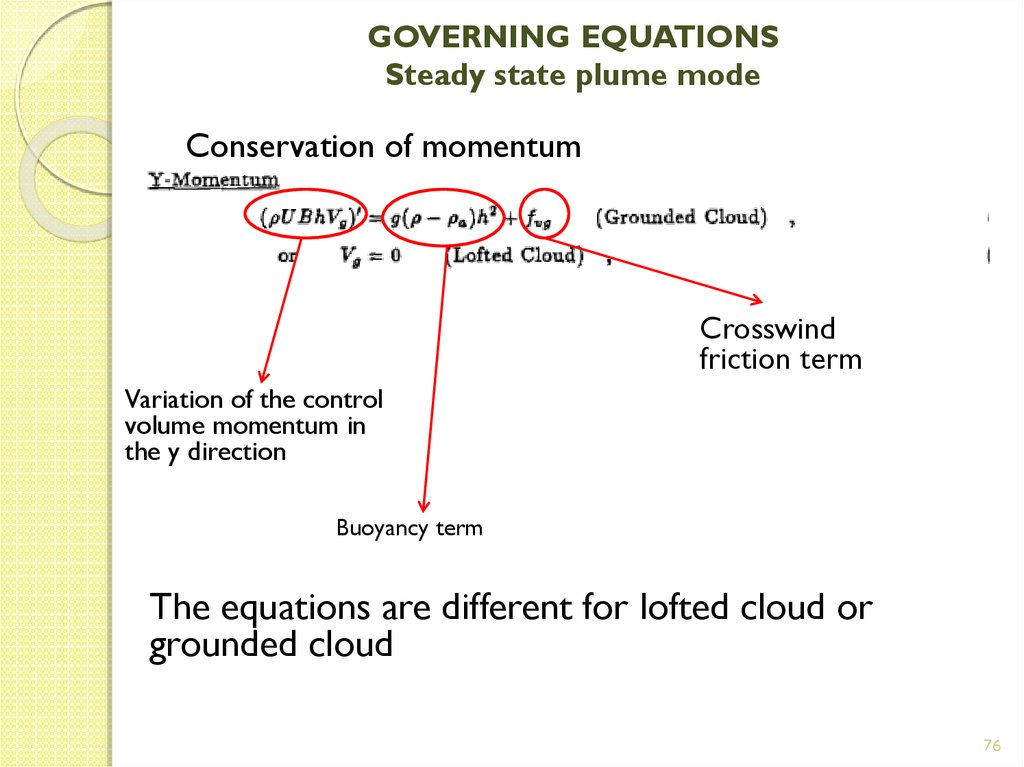
Conservation of momentum
Crosswind
friction term
Variation of the control
volume momentum in
the y direction
Buoyancy term
The equations are different for lofted cloud or
grounded cloud
76

77. GOVERNING EQUATIONS Steady state plume mode

Conservation of momentum
Friction term
Variation of the control
volume momentum in
the z direction
Buoyancy term
77

78. GOVERNING EQUATIONS Steady state plume mode

In a horizontal jet release, the source velocity term Ws = 0
(in the z direction) everywhere. The jet is treated as an
elevated area source pointing in the downwind direction with
the jet center located at the downwind distance x = 1m and
z = hs.
In a vertical jet release the source is treated as an elevated
area source pointing upwards with x = y = 0 and z = hs.
The plume rise portion of the cloud dispersion is calculated
in a separate submodel .
In the steady state plume region, gravitational falling of the
plume occurs if the cloud is denser than air and it is elevated
above ground.
78

79. GOVERNING EQUATIONS Steady state plume mode

The solution of the governing equations is divided into two
regions for the evaporating pool release. These regions are
the source region, where Ws > 0 (vertical jet velocity) and
the near field steady state region beyond the source where
Ws = 0.
The reason for this separation is that gravity spread of the
denser-than-air cloud manifests differently in the two regions.
79

80. GOVERNING EQUATIONS Transient puff mode

The transient puff mode of SLAB is based upon the volumeaveraged conservation equations of mass, momentum, energy
and species;
As before, it uses the air entrainment concept to account for
turbulent mixing of the cloud with the surrounding
atmosphere
The cloud is treated as a puff (see next page) and the
independent variable is the downwind travel time t of the
puff center of mass
80

81. GOVERNING EQUATIONS Transient puff mode

81

82. GOVERNING EQUATIONS Transient puff mode

82

83. GOVERNING EQUATIONS Transient puff mode

The equations for the puff mode differ from those in the
plume mode for the fact that the variation of the mass,
energy, momentum and species is a variation with time
instead of a variation with the x direction.
This is because in the puff mode the system is no more
stationary, but it proceeds forward in the space changing its
position and its volume with time.
Equation 22 in fact describes the position of the cloud center
of mass in function of its geometry and of the source term.
83

84. GOVERNING EQUATIONS Transition from plume to puff mode

The puff dispersion mode can be entered:
at the beginning of a simulation by specifying an instantaneous or
short duration evaporating pool source;
Or in the middle of a simulation after the release is completed and
the steady state period is over.
In the latter case there is a transition in the calculation of the
spacially-averaged cloud properties from the steady state plume
equations to the transient puff equations.
In the plume mode the equations are averaged over the crosswind
plane of the cloud
In the puff mode they are averaged over the cloud volume.
84

85. GOVERNING EQUATIONS Transition from plume to puff mode

To begin the puff mode calculation it is necessary to define
the time of this transition and the cloud length and the
center of mass at this time.
The transition time is taken to occur at the end of the
release, when t = t_sd.
The downwind location of the cloud center of mass Xc(t_sd)
is obtained by calculating the total mass of the released
material within the cloud as a function of downwind distance.
The cloud center of mass is taken to be the downwind
location at which the mass of released material from the
upwind edge to the center of mass is equal to ½ of the total
amount of material released.
85

86. GOVERNING EQUATIONS Cloud length and time dependence in the plume mode

The approach taken in the previous section for the
calculation of the cloud center of mass and half length at the
transition plume-puff can be extended to a calculation of the
properties for any time during the release, 0<t<t_sd.
The cloud center of mass is defined as the downwind
distance at which the mass of released material from the
upwind edge to the center of mass is equal to ½ the material
released during time t.
86

87. GOVERNING EQUATIONS Solution of the dispersion equations

The basic model equations can be solved by direct
numerical integration of the equations as given in the
previous subsections.
However, analytic solutions to some of these equations can
be obtained by rearranging the equations and defining new
variables.
This approach is used in SLAB since it presumably will
provide more accurate results.
87

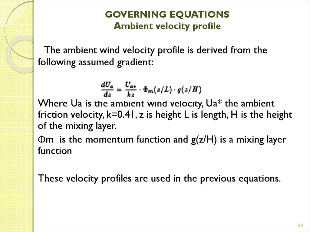
88. GOVERNING EQUATIONS Ambient velocity profile

The ambient wind velocity profile is derived from the
following assumed gradient:
Where Ua is the ambient wind velocity, Ua* the ambient
friction velocity, k=0.41, z is height L is length, H is the height
of the mixing layer.
Φm is the momentum function and g(z/H) is a mixing layer
function
These velocity profiles are used in the previous equations.
88

89. GOVERNING EQUATIONS Entrainment rates

The vertical entrainment rate includes the effects of surface
friction, differential motion between air and cloud, thermal
convection due to ground heating, damping of air-cloud
mixing due to stable density stratification within the cloud.
The formula used in SLAB is based on experimental data
from several sources.
89

90. GOVERNING EQUATIONS Heat and momentum flux terms

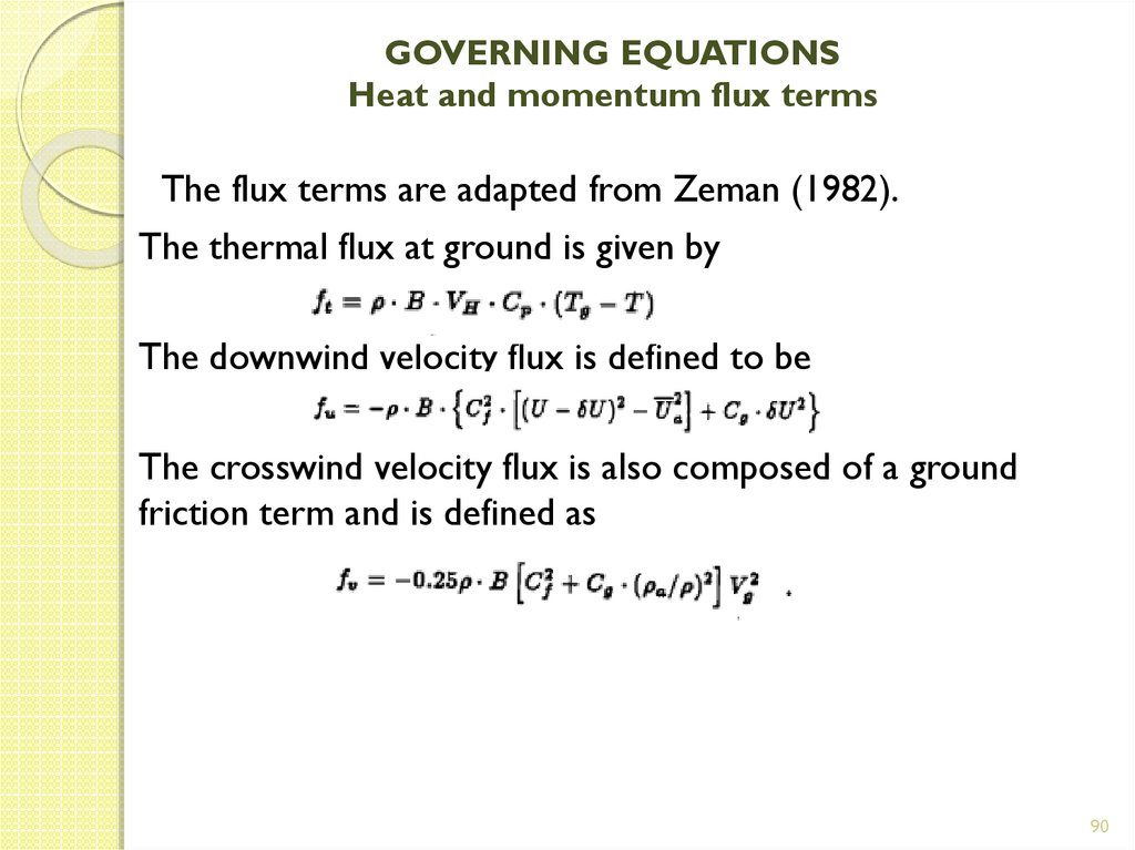
The flux terms are adapted from Zeman (1982).
The thermal flux at ground is given by
The downwind velocity flux is defined to be
The crosswind velocity flux is also composed of a ground
friction term and is defined as
90

91. GOVERNING EQUATIONS Thermodynamic model

Liquid droplets formation and evaporation is governed by an
equilibrium thermodynamic model in SLAB.
Two species are allowed to form droplets: the ambient water
vapor that enters the cloud and the released emission within the
cloud.
The governing equations are:
the mass conservation equation for the released material
additional mass conservation equations for the dry air, total
water and the liquid-vapor fractions of water and emission
the energy conservation
the equation of state for a liquid droplet-vapor mixture
the equilibrium condition that controls the liquid-vapor ratio for
each species.
91

92. GOVERNING EQUATIONS Plume rise

The plume from a vertical jet or stack release initially rises
until a maximum plume height is attained.
In SLAB the plume rise region is obtained from the results of
wind tunnel and field experiments.
Three types of jet are considered:
denser than air jets (ρs>ρa)
momentum jets (ρs=ρa)
buoyant jets (ρs<ρa)
92

93. TIME AVERAGED CONCENTRATIONS

All of the SLAB results (concentration, cloud width …)
represent ensemble averages.
An ensemble average is an average over numerous experiments
under the same conditions.
In a dispersion experiment these conditions are the spill terrain,
and meteorological conditions.
Since the model predicted concentration is an ensemble average,
it may be greater than or less than the measured concentration.
The situation is depicted in the next page, where the
instantaneous concentration at time t and downwind distance x
is compared with the ensemble average.
93

94. TIME AVERAGED CONCENTRATIONS

94

95. TIME AVERAGED CONCENTRATIONS

in addition to the ensemble average, SLAB uses two other
average types:
Spatial averages which are used in the dispersion equations
to simplify them.
Time averages which are averages taken at a particular
location (x,y,z) over a duration of time t_av, called concentration
averaging time.
The reason for time averaging is that safety levels for hazardous
chemicals are generally expressed as a maximum allowable
average concentration level for a given time exposure.
In SLAB the concentration averaging time is an input data.
95

96. Cloud meander

Cloud meander is the random oscillation of the cloud
centerline about the mean wind direction as shown in the next
image.
96

97. Cloud meander

When the cloud concentration os averaged over time, the
effective width of the cloud appears to be wider due to the
wandering of the cloud centerline.
In addition, the mean cloud concentration decreases in the
region about the mean centerline.
Empirically, it has been found that the effective width of the
cloud increases as the concentration averaging time is increased
(see figure in previous page)
97

98. Cloud meander

In SLAB code solution to the dispersion equations, the cloud
meander is ignored and the cloud is assumed to travel in a
straight line.
Consequently, in terms of time averaging, these results are the
“instantaneous” average obtained in absence of cloud meander.
To include the effects of cloud meander the “instantaneous”
average cloud needs to be modified to include the cloud width
due to the displacement y0 (see figure) of the meandering cloud
centerline about the mean wind direction.
98

99. Time averaged volume concentration

With the determination of the effective cloud half width for
the concentration averaging time t_av, the calculation of the
time-averaged cloud properties is easily accomplished.
In SLAB, the only calculated time-averaged property is the
volume concentration expressed as the volume fraction with
values from 0 to 1.
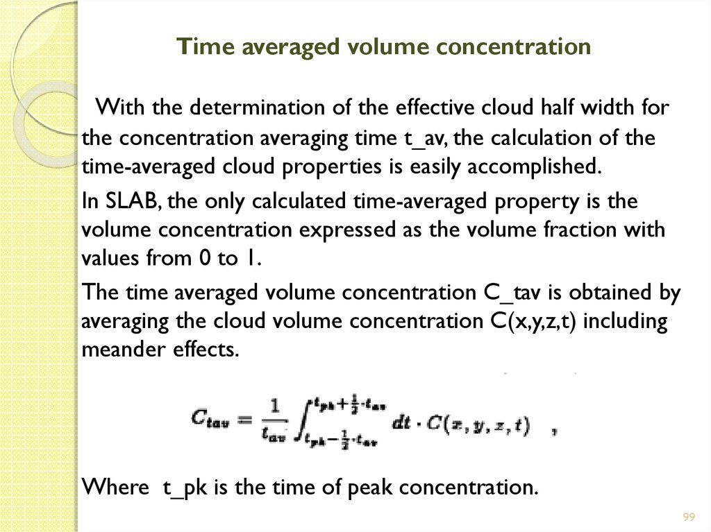
The time averaged volume concentration C_tav is obtained by
averaging the cloud volume concentration C(x,y,z,t) including
meander effects.
Where t_pk is the time of peak concentration.
99

100. SLAB User’s guide

100

101. General information

SLAB is implemented in the Fortran 77 language.
SLAB operates by acquiring an input data file named INPUT
containing the input parameters.
A SLAB problem may consist of a single run or several runs
where metereologic conditions can vary while the remainder of
the spill scenario is the same.
SLAB produces as output a file named PREDICT containing the
output from a single problem which may include one or more
SLAB runs.
101

102. Input file

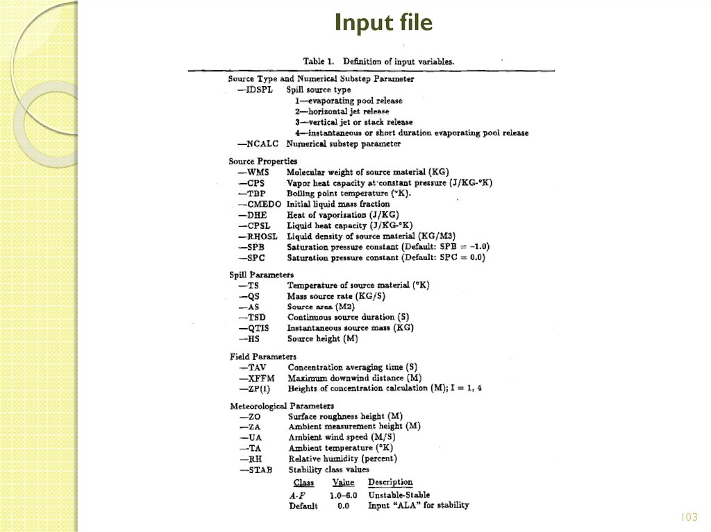
There are 30 possible input parameters required to run in
SLAB.
Such parameters include the source type, source properties,
spill properties, field properties, meteorological parameters and
a numerical substep parameter.
These input parameters define uniquely the problem.
The table in the next page lists the input parameters.
102

103. Input file

103

104. Source type and numerical substep parameter

IDSPL – Spill source type
SLAB has 4 types of sources identified by the integer 1 – 4.
Evaporating pool release
2) Horizontal jet release
3) Vertical jet or stack release
4) Instantaneous or short duration evaporating pool release
1)
These 4 kinds of sources are schematized in the next figure 5.
104

105. Source type and numerical substep parameter

Figure 5
105

106. Source type and numerical substep parameter

The evaporating pool is a ground level area source of finite
duration TSD. The source is located at the axes origin.
When the spill duration is short enough a steady state plume
will not form.
In this case the code automatically stops and redefines the
source type to “short duration evaporating pool release (IDSPL
= 4).
The horizontal jet release is an area source with jet center
located at x=1, y=0, z=HS.
The initial mass fraction is 1.0 with the initial liquid mass fraction
specified by the input parameter CMEDO.
The initial vapor mass fraction is thus 1 – CMEDO.
106

107. Source type and numerical substep parameter

The vertical jet release is an area source with source plane
parallel to the ground and source velocity pointing upward.
The same considerations as the horizontal jet can be done for
the mass fraction.
The instantaneous or short duration evaporating pool
release is a combination of two sources: an instantaneous
volume source with a total mass given by the parameter QTIS
and a short duration, ground level area source with a source
rate and a spill duration given by the input parameters QS and
TSD respectively.
When an instantaneous volume release is simulated, QTIS is
specified and QS and TSD are set to zero.
107

108. Source type and numerical substep parameter

In SLAB the pressure within the cloud is always 101325 Pa. If
an explosion is to be simulated the SLAB calculation begins after
the source is fully expanded to atmospheric pressure.
It is recommended that an evaporating pool release of any finite
duration be run in the source type parameter with IDSPL = 1.
If the steady state cloud is not achieved, the code will turn
automatically into IDSPL = 4.
108

109. Source type and numerical substep parameter

The parameter NCALC is an integer substep multiplier that
specifies the number of calculation sub-steps performed during
the integration of the conservation equations.
A value of NCALC=1 is generally recommended to provide
computational stability and sufficient numerical accuracy
However, if stability problems rise, the value of NCALC can be
increased.
109

110. Source properties

WMS = molecular weight of the source material [kg]
CPS = vapor heat capacity at constant pressure [J/kgK]
TBP = boiling point temperature of source material [K]
CMEDO = Initial liquid mass fraction
The emission is assumed to be the pure substance with a
fraction CMEDO in liquid phase in the form of liquid droplets;
the remainder (1 – CMEDO) is in the vapor phase.
110

111. Source properties

DHE = heat of vaporization at the boiling point
temperature[J/kg]
CPSL = liquid specific heat of the source material[J/kgK]
RHOSL = liquid density of source material [kg/m3]
SBP-SPC = saturation pressure constants
The saturation pressure constants are used in the following
formula for the saturation pressure
Where PA is ambient pressure and T the local temperature.
111

112. Source properties

Some examples of substances are here provided
112

113. Spill parameters

TS = temperature of the source material
When the release is an evaporating pool, the source
temperature is the boiling point temperature TBP.
When the release is instantaneous (IDSPL=4) and the source is
the result of an explosion, TS is the temperature of the material
after it has fully expanded.
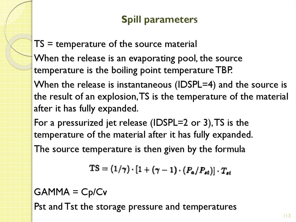
For a pressurized jet release (IDSPL=2 or 3), TS is the
temperature of the material after it has fully expanded.
The source temperature is then given by the formula
GAMMA = Cp/Cv
Pst and Tst the storage pressure and temperatures
113

114. Spill parameters

QS = mass source rate [kg/s]4
For an instantaneous release, the QS value should be set to
zero.
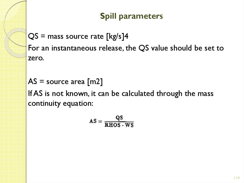
AS = source area [m2]
If AS is not known, it can be calculated through the mass
continuity equation:
114

115. Spill parameters

TSD = continuous source duration [s]
This parameter specifies the duration of the release from an
evaporating pool, (IDSPL=1 or 4) or jet (IDSPL = 2 or 3) source.
When an instantaneous release is to be simulated, TSD =0.
QTIS = instantaneous source mass [kg]
This is the total mass of the instantaneous release. For an evaporating
pool or jet should be equal to zero.
HS = source height [m]
For a pool, HS=0
For horizontal jet is the height at jet center
For an instantaneous release, the source area AS multiplied by the
height HS is equal to the total volume released.
115

116. Field parameters

TAV = concentration averaging time [s]
The concentration averaging time is the appropriate averaging
time for the safety standard of interest. E.G. if the safety
standard of interest for a particular material is a maximum
average concentration of 100 ppm for a 1h exposure, then
TAV=3600 s.
Care should be taken when TAV is greater than the cloud
duration TCD. In this case the average concentration will be
reduced since the puff is relatively short and the observer is
exposed to the material for only a fraction of the concentration
averaging time.
In this case, a more meaningful TAV value to use might be one
that is less or equal to the cloud duration.
116

117. Field parameters

XFFM=maximum downwind distance [m]
This is the maximum downwind (x) distance for which the user
is interested in knowing the cloud concentration.
In steady state plume mode, the simulation is conducted to a
downwind distance equal to XFFM. However, in the transient
puff dispersion mode, time is the independent variable rather
than distance.
Then, in puff mode the simulation is conducted to a downwind
distance a bit larger than XFFM.
ZP(I), I=1,4 = heights of concentration calculation
There are a maximum of 4 heights at which the concentration is
calculated as a function of downwind distance.
117

118. Meteo parameters

ZO = surface roughness height [m]
Is generally estimated in two ways:
The first method is to extrapolate measured ambient velocity
profile data under neutral stability conditions. This can be done
by a least square fit to determine the friction velocity U0 and
surface roughness height ZO.
The second method uses values of ZO that have been
empirically determined for various ground surface conditions, as
listed in the table below
118

119. Meteo parameters

ZA = ambient measurement height [m]
This is the height at which ambient windspeed is measured. This
height should be much larger than ZO.
UA = ambient wind speed [m/s]
TA = ambient temperature [K]
RH = relative humidity [%]
119

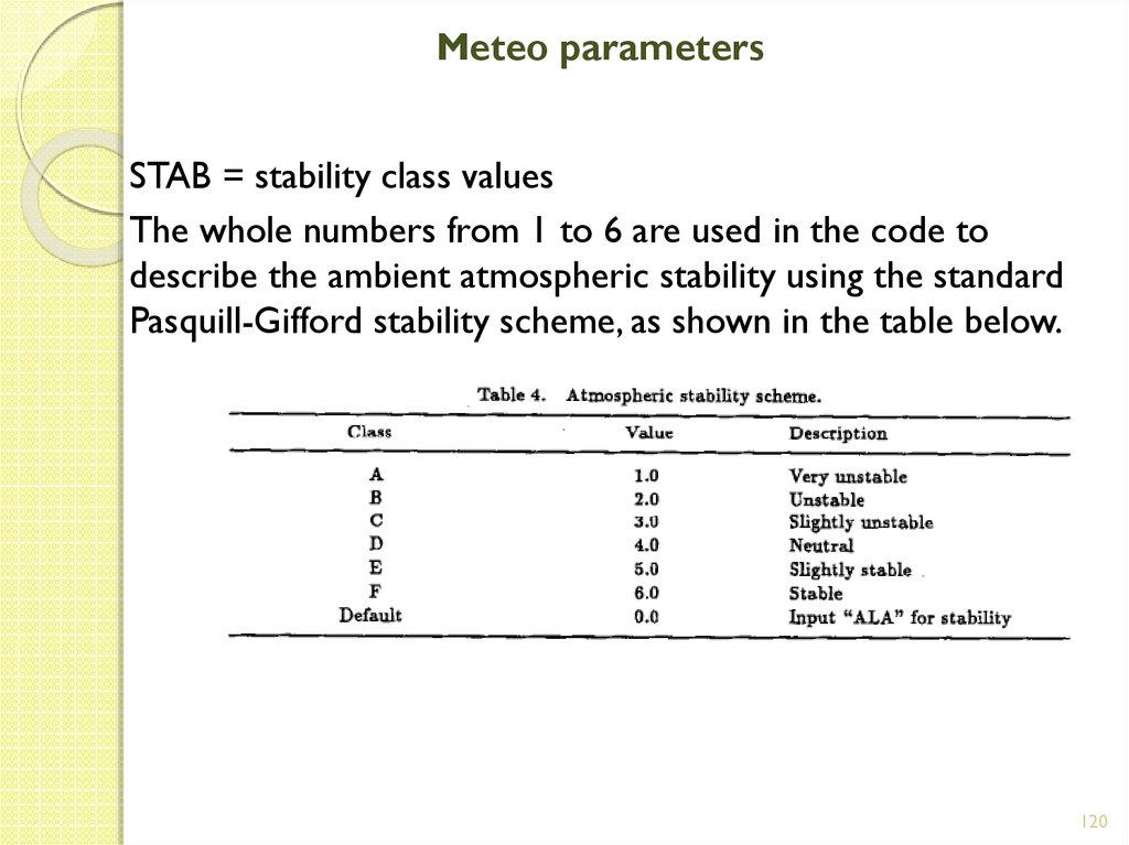
120. Meteo parameters

STAB = stability class values
The whole numbers from 1 to 6 are used in the code to
describe the ambient atmospheric stability using the standard
Pasquill-Gifford stability scheme, as shown in the table below.
120

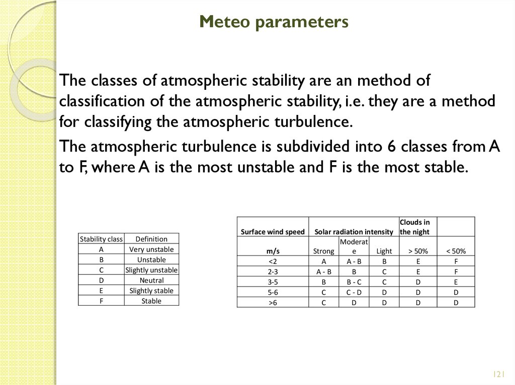
121. Meteo parameters

The classes of atmospheric stability are an method of
classification of the atmospheric stability, i.e. they are a method
for classifying the atmospheric turbulence.
The atmospheric turbulence is subdivided into 6 classes from A
to F, where A is the most unstable and F is the most stable.
Stability class
Definition
A
Very unstable
B
Unstable
C
Slightly unstable
D
Neutral
E
Slightly stable
F
Stable
Surface wind speed
m/s
<2
2-3
3-5
5-6
>6
Clouds in
Solar radiation intensity the night
Moderat
Strong
e
Light
> 50%
A
A-B
B
E
A-B
B
C
E
B
B-C
C
D
C
C-D
D
D
C
D
D
D
< 50%
F
F
E
D
D
121

122. Meteo parameters

ALA = inverse Monin-Obukhov length [1/m]
This is a stability parameter used to describe the vertical profile
of ambient wind speed and the vertical turbulent diffusivity.
This option for describing atmospheric stability is activated by
setting STAB=0.0. ALA is an input parameter only when
STAB=0.0. Inclusion of ALA when STAB is not zero results in an
error.
122

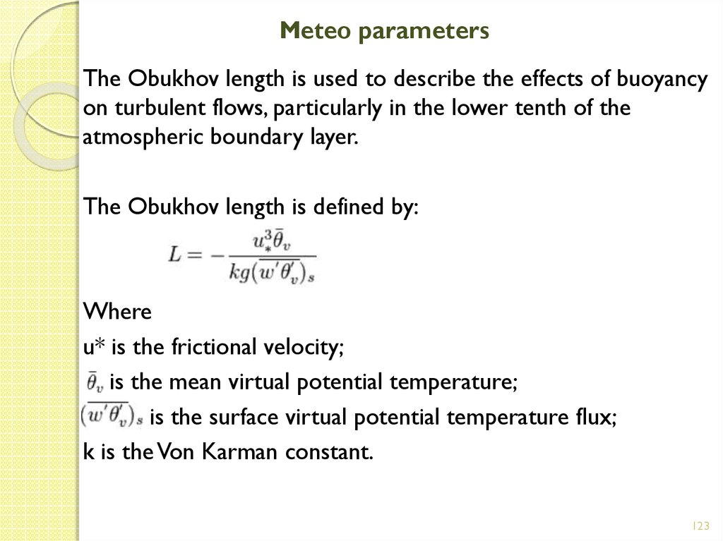
123. Meteo parameters

The Obukhov length is used to describe the effects of buoyancy
on turbulent flows, particularly in the lower tenth of the
atmospheric boundary layer.
The Obukhov length is defined by:
Where
u* is the frictional velocity;
is the mean virtual potential temperature;
is the surface virtual potential temperature flux;
k is the Von Karman constant.
123

124. Input file closure

After the code has read the input and executed a run, it returns
to the start of the code looking for an additional value of ZO
(surface roughness height) .
If an additional value of ZO is specified, the code will look for
the remaining meteo input parameters (ZA, UA, TA, RH, STAB,
ALA) and executes an additional run with the new metrologicla
inputs.
In this way multiple runs can be made with the same source, but
different meteo conditions.
When the code looks for an additional value of ZO and finds a
value minor than zero, it terminates the problem.
Thus the problem is terminated by including an additional input
parameter with the value -1.
124

125. CALCULATIONAL FLOW

A SLAB model simulation can be viewed as occurring in three
sequential phases: initialization, sequential calculation and time
averaged concentration calculation.
The calculational flow starting with the identified source type
and ending with the calculation of the time averaged
concentration as shown in the figure below.
125

126. CALCULATIONAL FLOW Initialization

The initialization begins with the specification of the
source type.
There is one case where the code overrides the specified
source type, that is when “evaporating pool” is specified
and the release duration is so short that a steady state
cloud is not reached. In this case, the source type is
switched to “instantaneous or short duration release”.
126

127. CALCULATIONAL FLOW Dispersion calculation

The dispersion phase contains the bulk of the calculation. It is
here that the conservation and thermodynamic equations are
solved, yielding the instantaneous (no meander) spacially
averaged properties in function of downwind distance.
There are two dispersion modes: plume and puff., of which a
sketch is given in the picture below
127

128. CALCULATIONAL FLOW Dispersion calculation

The steady state plume mode is used for the finite duration
releases until the end of the release.
After the release is over, the transient puff mode is used for
the remainder of the simulation.
The transient puff mode is also used in the case of an
instantaneous release or when the release is so short that a
steady state is not reached.
These two models represent two different forms of the
conservation equations.
128

129. CALCULATIONAL FLOW Dispersion calculation

In the steady state plume mode the conservation equations
are spatially averaged over the cross-wind plane of the cloud,
as visible in the picture at page 78.
Consequently, the resulting cloud properties are also spatially
averaged over the crosswind plane.
Thus, the relation between concentration C(x,y,z) and the
cross averaged concentration C(x) is given by:
Where B and h are the cloud half width and height.
The crosswind averaged concentration is not expressed as a
function of time since the plume is considered in steady state.
129

130. CALCULATIONAL FLOW Dispersion calculation

In the transient puff mode the conservation equations are
averaged over the entire volume of the cloud.
Consequently, the solution yields volume-averaged properties.
So, the relationship between the concentration C(x,y,z,t) and
the volume-averaged concentration C(t) is given by:
Where B, Bx and h are the cloud half width, half length and half
height.
These parameters and the cloud center of mass are calculated
along with the solution of the conservation equations.
130

131. CALCULATIONAL FLOW Dispersion calculation

In the transient puff mode the conservation equations are
averaged over the entire volume of the cloud.
Consequently, the solution yields volume-averaged properties.
So, the relationship between the concentration C(x,y,z,t) and
the volume-averaged concentration C(t) is given by:
Where B, Bx and h are the cloud half width, half length and half
height.
These parameters and the cloud center of mass are calculated
along with the solution of the conservation equations.
131

132. CALCULATIONAL FLOW Time averaged concentration calculation

After the spatially-averaged cloud properties are calculated at all
downwind distances, the code calculates the time averaged
concentration.
In SLAB, the concentration is expressed as the volume fraction,
ranging from 0 to 1.
The time-averaged volume fraction C_tav(x,y,z,t) is calculated by the
spatially averaged volume fraction C(Xc,t) and the cloud height,
width and length parameters.
To do this, the concentration distribution about the center of mass
Xc must be assumed since C(Xc,t) does not contain this
information.
SLAB uses profile distribution functions, which are functions of the
calculated half width, half length and height of the cloud.
132

133. CALCULATIONAL FLOW Time averaged concentration calculation

The calculation of the time averaged volume fraction
C_tav(x,y,z,t) from the volume fraction C(x-Xc,y,z,t), involves
two steps:
1) The calculation of the cloud half-width
2) The calculation of the time averaged volume fraction
The effects of the cloud meander is to increase the width of
the cloud, reducing the average concentration observed in the
cloud centerline region.
The longer the averaging time, the more meander can occur
and the greater the increase in the effective width.
133

134. CALCULATIONAL FLOW Time averaged concentration calculation

The time available for cloud meander at the downwind
location x cannot be longer than the duration of the exposure
to the cloud at the same location.
Thus, the time available for cloud meander is assumed to be
equal to the concentration averaging time t_av with a
maximum value equal to the cloud duration t_cd.
As a result, the cloud effective width increases monotonically
with the concentration averaging time t_av until some
maximum value is reached that is dependent on the length of
the cloud.
With the calculation of the cloud effective half width, the time
averaged volume fraction can now be determined.
The calculation of the time averaged volume fraction
concludes the SLAB run.
134

135. OUTPUT FILE

The output file contains several types of information which can
be grouped in 3 categories:
1) Problem description
2) Instantaneous spatially averaged cloud properties
3) Time averaged volume fraction
These categories correspond to the three sequential phases
(initialization, dispersion calculation and time-averaged
concentration calculation) of the SLAB code calculation.
135

136. OUTPUT FILE Problem description

The Problem description output lists the various input
parameters used by the code and thereby defines the problem
to be solved.
The first group is the problem input parameter values as
specified by the user.
Some input parameters (IDSPL, SPB, SPC, TS and STAB) may be
changed by the code in order to be consistent with SLAB
model assumptions.
136

137. OUTPUT FILE Instantaneous spatially averaged cloud properties

The instantaneous spatially averaged cloud properties output
gives the results of the dispersion calculation phase of the
simulation.
These results are intermediate results in that they are the
solution of the spatially averaged (plume or pluff)
conservation equations, the equation of state and the length
and width equations.
However they do not include the effects of cloud meander
time averaging.
137

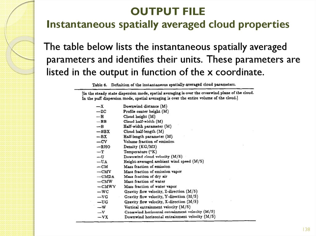
138. OUTPUT FILE Instantaneous spatially averaged cloud properties

The table below lists the instantaneous spatially averaged
parameters and identifies their units. These parameters are
listed in the output in function of the x coordinate.
138

139. OUTPUT FILE Instantaneous spatially averaged cloud properties

The cloud properties listed before, are described as
“instantaneous” and “spatially” averaged properties.
All of the SLAB results are ensemble average values: they
represent the average taken over numerous trials under the
same conditions.
In addition, these ensemble average values can be averaged over
time and space.
The term “instantaneous” refers to the time averaging and
indicates that the duration of the time period over which the
average is taken is essentially zero.
Thus the effects of cloud meander are assumed to be absent in
the “instantaneous” average.
139

140. OUTPUT FILE Instantaneous spatially averaged cloud properties

The “spatial” averaging in SLAB is of 2 types: cross-wind and
volume average.
The choice of the spatial average depends on the dispersion
mode (plume or puff).
When a finite duration release is simulated, a transition occurs
in the dispersion calculation as the code switches from the
plume to the puff mode, with the transition occurring at the
end of the release, t = TSD.
Since there is no discontinuity in the actual dispersion of the
cloud at this time, the code predicted values should also
maintain this continuity.
This is done in SLAB by the definition of the cloud half length at
the time of the transition in the dispersion mode calculation.
140

141. OUTPUT FILE Time averaged volume fraction

In SLAB the time averaged concentration is expressed as the
time averaged volume fraction with values ranging from 0 to 1.
This is easily turned into ppm concentration
multiplying by one million.
The time average volume concentration output is is presented
under 3 sub titles:
1) Concentration contour parameters
2) Concentration in the Z = ZP(I) plane (height of
concentration calculation)
3) Maximum centerline concentration
All of these results are presented from the point of view of an
observer located at the downwind distance x, crosswind
distance y and height z above the ground.
141

142. OUTPUT FILE Time averaged volume fraction

The concentration contour parameters output lists a number of
parameters from which the time-averaged volume
concentration at any downwind location and time within the
problem domain can be calculated.
142

143. OUTPUT FILE Time averaged volume fraction

The concentration in the Z=ZP(I) plane gives the the time
averaged volume concentration in the horizontal plane at the
height ZP(I) above ground.
Up to four planes can be selected by the user, all of which are
specified in the input.
In the output, concentration is listed in function of downwind
distance x.
At each downwind distance, the time of maximum
concentration, cloud duration and effective cloud half-width is
given.
143

144. OUTPUT FILE Time averaged volume fraction

The final result is the maximum centerline concentration.
Here the maximum time averaged volume concentration along the
cloud centerline is given as a function of the downwind distance x
and the height Z_pk at which the maximum occurs.
Generally, Z_pk = 0 except when the source is elevated or the cloud
becomes positively buoyant and begins to loft.
In the output, at each specified downwind location, the code lists the
height at which the maximum occurs, the maximum time averaged
volume concentration expressed as a volume fraction from 0 to 1,
the time of maximum concentration and the cloud duration.
144

145. CONCLUDING REMARKS

Two cautions are given regarding the use of SLAB
predicted values of the time-averaged concentration.
1) The comparison of the model predictions with safety
standards for a hazardous material
2) The comparison of model prediction with actual
experiments.
Safety standards are given as a maximum average
concentration for a specified exposure duration.
145