Modeling non-stationary variables

1.

Modeling Non-stationary Variables
Joint Vienna Institute/ IMF ICD
Macro-econometric Forecasting and Analysis,
JV16.12, L02, Vienna, Austria, May 17, 2016
Presenter
Mikhail Pranovich
This training material is the property of the International Monetary Fund (IMF) and is intended for use in
IMF’s Institute for Capacity development (ICD) courses. Any reuse requires the permission of ICD.

2.

Lecture Objectives
• Revisit the concept of non-stationary (unit root) process and
its implications for analysis and forecasting
• Understand key tests for unit root
• Revisit the concept of cointegration
• … and testing for cointegration
2

3. Outline

Stationary and non-stationary variables
Testing for unit roots
Cointegration
Testing for cointegration
3

4. Introduction

Many economic (macro/financial) variables exhibit trending
behavior
e.g., real GDP, real consumption, assets prices, dividends…
Key issue for estimation/forecasting:
the nature of this trend….
… is it deterministic (e.g., linear trend) or stochastic (e.g., random
walk)
The nature of the trend has important implications for the
model’s parameters and their distributions…
… and thus for the statistical procedures used to conduct
inference and forecasting
4
Macro-econometric Forecasting and
Analysis

5. Key Macro Series Appear to have trends

Share Prices
Exchange Rate
4.75
15
Real GDP
14
GDP Deflator
4.50
4.25
4.00
13
3.75
3.50
12
3.25
11
3.00
2.75
10
1950
5
1955
1960
1965
1970
1975
1980
1985
1990
1995
2000
1950
1955
1960
1965
1970
Macro-econometric Forecasting and
1975
1980
1985
1990
1995
2000

6. Deterministic and Stochastic Trends in Data

Two types of trends: deterministic or stochastic
A Deterministic trend is a non-random function of time
Example: linear time-trend
y t 1 2 t εt
A stochastic trend is random, i.e. varies over time
Examples:
(Pure) Random Walk Model: a time series is said to follow a pure random walk if
the change is i.i.d.
yt yt 1 εt
Random Walk with a Drift
yt yt 1 εt
is a ‘drift’. If > 0, then yt increases on average
6

7. Example: Processes with Trends

60
40
Deterministic trend
Stochastic trend
35
50
30
40
25
30
20
15
20
10
10
5
0
0
20
40
60
80
100
120
140
160
180
200
0
20
40
60
80
100
120
140
160
7
180
200

8. Stationary and non-stationary processes (1)

Consider the data generation process (DGP)
y qy t
t
t 1
1.0, variable is stationary (i.e.,
If q <the
mean and variance)
Standard econometric procedures may be used to
estimate/forecast this model
8
Macro-econometric Forecasting and
Analysis
yt finite
, has

9.

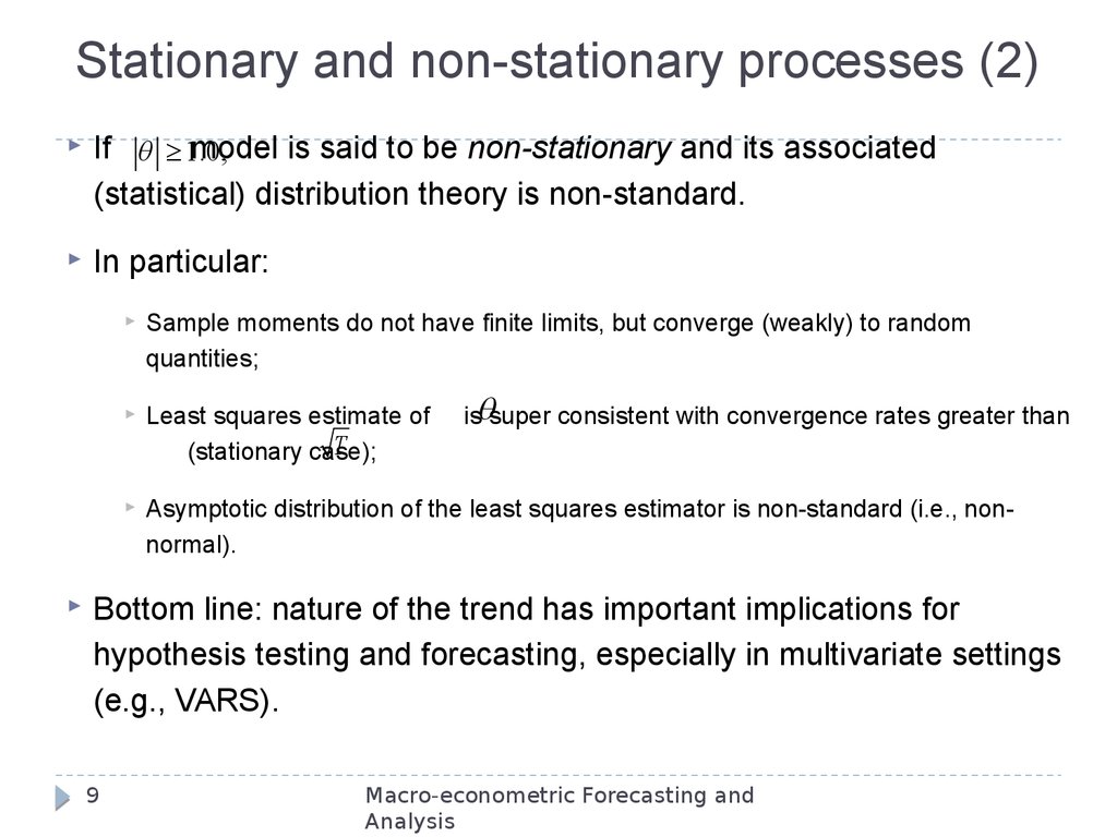
Stationary and non-stationary processes (2)
If q ³ 1.0,
model is said to be non-stationary and its associated
(statistical) distribution theory is non-standard.
In particular:
Sample moments do not have finite limits, but converge (weakly) to random
quantities;
Least squares estimate of
T
(stationary case);
Asymptotic distribution of the least squares estimator is non-standard (i.e., nonnormal).
isqsuper consistent with convergence rates greater than
Bottom line: nature of the trend has important implications for
hypothesis testing and forecasting, especially in multivariate settings
(e.g., VARS).
9
Macro-econometric Forecasting and
Analysis

10. Reminder: Autoregressive AR(p) Process

We shall check how shocks affect stationary and non-
stationary variables, but first recall what is an AR(p) process
An AR(p) autoregressive process (AR-process of order p):
y t q1 y t 1 q 2 y t 2 ... q p y t p εt
The error εt, is assumed to be independently and identically
distributed (i.i.d.), with a zero mean and a constant variance
10

11. Stochastic trends, autoregressive models and a unit root

The condition for stationarity in an AR(p) model: roots z of the
characteristic equation
1- θ1z - θ2z2 - θ3z3 - ... - θpzp =0
must all be greater than one in absolute value: |z| >1
If an AR(p) process has z=1 => variable has a unit root
Example: AR(1) process yt =
+ θyt-1 + vt
A special case is θ =1 => z =1 => yt has unit root (stochastic trend)
Stationarity requires that |θ| <1 for |z|>1
11

12. The Impact of Shocks on Stationary and Non-stationary variables

Consider a simple AR(1):
yt = θyt-1 + νt,
where θ takes any value for now
We can write:
yt-1= θyt-2 + νt-1
yt-2= θyt-3 + νt-2
Substituting yields:
yt = θ(θyt-2 + νt-1) + εt = θ2yt-2 + θνt-1 + νt
Successive substituting for yt-2, yt-3,... gives an representation in terms of
initial value y-1 and past errors νt-1, νt-2,...,ν0
yt = θt+1y-1 + θνt-1 + θ2νt-2 + θ3νt-3 + ...+ θtν0 + νt
12

13. The Impact of Shocks for Stationary and Non-stationary Series (2)

Representation at t=T: yT = θT+1y-1 +θvT-1 +θ2vT-2 + θ3vT-3 + ...+ θTv0 + vT
At t =0 the variable is hit by a non-zero shock
We have 3 cases (depending on value of θ):
1.
v0
|θ|< 1 θT 0 and θTv0 0 as T
Shocks have only a transitory effect (gradually dies away with time)
2.
θ = 1 θT = 1 and θTv0 = v0 T
Shocks have a permanent effect in the system and never die away:
T
yT y 1 vi
i 0
... just a sum of past shocks plus some starting value of y-1. The
grows without bound (Tσ2 ) as T
3.
variance
|θ|>1. Now shocks become more influential as time goes on (explosive
effect), since if θ>1, then |θ|T>...>|θ|3 > |θ|2 > |θ| etc.
13

14. Integration

Another way to write the stochastic trend model is:
y y
t
t
y
t 1
t
Thus the first difference of yt is stationary provided vt is
stationary (“difference stationary” process). Also
referred to as an I(1) variable.
Similarly, in the case of the deterministic trend model, yt
is interpreted as trend stationary
14
because removal of the deterministic trend from yt renders it
a stationary random variable
Macro-econometric Forecasting and
Analysis

15. Order of Integration: I(d)

In general, if yt is I(d) then:
d y (1 L) d y t
t
t
If d=0, then the series is already stationary
15
Macro-econometric Forecasting and
Analysis

16. Problems due to Stochastic Trends (from a statistical perspective)

Non-standard distribution of test statistics
Spurious regression:
in a simple linear regression, two (or more) non-stationary time series
may appear to be related even though they are not
Need to use special modeling techniques when dealing with
non-stationary data (VARs in differences or VECMs)
Need to distinguish btw. stochastic and deterministic trends as
it may affect estimates of policy-relevant variables
e.g. estimate of an output gap or of a structural budget deficit
… for that we need unit root tests…
16

17. Figure 5: Distribution of OLS estimator for θ

17
Macro-econometric Forecasting and
Analysis

18. Testing For Unit Roots

Previous section suggests that I(1) variables need
special handling
So how do we identify I(1) processes, i.e., test for
unit roots?
Natural test is to consider the t-statistic for the nullhypothesis of a unit root, i.e., qˆ 1
Given the previous graph, it is not surprising that the
t-distribution for qˆ 1 is non-normal
18
Macro-econometric Forecasting and
Analysis

19. Testing for Unit Roots: Procedures

Dickey Fuller
Augmented Dickey Fuller
Phillips Perron
Kwiatkowski, Phillips, Schmidt and Shin (KPSS)
19
Macro-econometric Forecasting and
Analysis

20. Dickey Fuller Test

Fuller (1976), Dickey and Fuller (1979)
Example:
consider a particular case of an AR(1) model:
yt = θyt-1 + εt
We test a hypothesis
H0: θ =1 → the series contains a unit root/stochastic trend (is a random
walk)
against
H1: |θ| <1 → the series is a zero-mean stationary AR(1)
20

21. Dickey-Fuller Test (2)

For the purpose of testing we reformulate the regression:
yt = yt – yt-1 =θyt-1 -yt-1 + vt = (θ-1)yt-1 + vt =
= yt-1 + vt
so that the test of H0: θ = 1 H0: = 0
The test is based on the t-ratio for
this t-ratio does not have the usual t-distribution under the H0
critical values are derived from Monte Carlo experiments, and are tabulated
(known): see appendix A
The test is not invariant to the addition of deterministic
components (more general formulation: intercept + time-trend)
21

22. Dickey-Fuller Test (3)

Important issue – shall deterministic components be included in the test model for
yt. Is this
yt = yt-1 + vt
or
yt = 1+ yt-1 + vt
or
yt = 1+ 2t+ yt-1 + vt ?
Two ways around:
Use prior information/assume whether the deterministic components are included, i.e. use
the restrictions (easy to implement in Eviews):
1≠0 and 2≠0
1≠0 and 2=0
1=0 and 2=0
Allow for uncertainty about deterministic components (more complicated in Eviews) and
implement a testing strategy to find out:
restrictions on deterministic components
if yt is non-stationary
22

23. DF-Test (3): Deterministic Components are Known

Say, we assume yt includes an intercept, but not a time trend
yt = 1+ θyt-1 + vt
We test a hypothesis:
H0: θ =1 → the series has a unit root/stochastic trend
against
H1: |θ| <1 → the series is zero-mean stationary AR(1)
Reformulate:
yt = 1+ yt-1 + vt
Test H0: =0 → the series has a unit root (stochastic trend) against
H1: < 0 → the series has no unit root (is stationary)
This way is easy – it is ready for you in Eviews
But, there are risks involved...
23

24. DF-Test (4): Risks Posed by Deterministic Components

If deterministic components are not included in the test, when
they should be, then the test is not correctly sized:
If deterministic components are included but they should not be,
then the test has low power (especially in finite (short) samples):
The test will reject the H0: =0, although it is in fact true and should not
be rejected (yt is non-stationary) – type I error
The test will not reject the H0: =0, although it is false and must be
rejected (yt is stationary) – type II error
This is why we may prefer (a degree of) uncertainty about
deterministic components and use testing strategies (see appendix
A for details):
Enders Strategy
Elder and Kennedy Strategy
24

25. The Augmented Dickey Fuller (ADF) Test

2
The DF-test above is only valid if εt is a white noise: εt i.i.d (o, )
εt will be autocorrelated if there was autocorrelation in the first
difference ( yt), and we have to control for it
The solution is to “augment” the test using p lags of the
dependent variable. The alternative model (including the
constant and the time trend) is now written as:
p
y t 1 2 t y t 1
a y
i
t i
εt
i 1
25

26. The ADF-Test (2)

Again, we have three choices:
(1) include neither a constant nor a time trend
(2) include a constant
(3) include a constant and a time trend
Again, we either:
use prior information and impose a model from the beginning, or
remain uncertain about deterministic components and follow one of the
Strategies
Useful result: Critical values for the ADF-test are the same as for
DF-test
Note, however, that the test statistics are sensitive to the lag length p
26

27. The ADF-Test: Lag Length Selection

Three approaches are commonly used:
Akaike Information Criterion (AIC)
Schwarz-Bayesian Criterion (SBC)
General-to-Specific successive t-tests on lag coefficients
AIC and BIC are statistics that favour fit (smaller residuals) but penalize for every
additional parameter that needs to be estimated:
So, we prefer a model with a smaller value of a criterion statistic
General-to-Specific: begin with a general model where p is fairly large, and
successively re-estimate with one less lag each time (keeping the sample fixed)
It is advised to use AIC
Tendency of SBC to select too parsimonious of a model
The ADF-test is biased when any autocorrelation remains in the residuals
27length
Note: the test critical values do not depend on the method used to select the lag

28. Dickey-Fuller (and ADF) Test: Criticism

The power of the tests is low if the process is stationary but
with a root “close” to 1 (so called “near unit root” process)
e.g. the test is poor at rejecting θ = 1 (ψ=0), when the true
data generating process is
yt = 0.95yt-1 + εt
This problem is particularly pronounced in small samples
28

29. The Phillips Perron (PP) test

Rather popular in the analysis of financial time series
The test regression for the PP-tests is
yt 1 2 t yt 1 t
PP modifies the test statistic to account for any serial correlation and
heteroskedasticity of εt
The usual t-statistic in the DF-testt 0
… is modified:
1
ˆ 2
T
T
…
2
2
2
ˆ
1 ˆ ˆ T SE ( ˆ )
Zt
t 0
2
ˆ2
ˆ2
2
ˆ
ˆt2 estimate of variance
1/ 2
t 1
q
T
j
1
ˆ 2 [1
] ˆ j , ˆ j
ˆt ˆt j estimate of autocovariance of order j ,
q 1
T t j 1
j 1
ˆ2
2
q is a number of lags, up to which errors autocorrelation might be present
29

30. The PP test (2)

Under the null hypothesis that ψ = 0, Zt statistic has the same
asymptotic distribution as the ADF t-statistic
Advantages:
PP-test is robust to general forms of heteroskedasticity in εt
No need to specify the lag length for the test regression
30

31. The Kwiatkowski-Phillips-Schmidt-Shin (KPSS) test

The KPSS test is a stationarity test. The H0 is: yt ~I(0)
Start with the model:
yt Dt t t
t t 1 ut , ut i.i.d (0, u2 ),
Dt contains deterministic components, εt is I(0) and may be heteroskedastic
2
2
0
The test is then H0: u
against the alternative H1: u 0
The KPSS test statistic is:
T
t
KPSS T 2
t 1
Sˆt2 / ˆ2
ˆ2
where
is a cumulative residual function and
is a
j 1
long-run variance of εt as defined earlier (see slide 32)
Sˆt uˆ j
See Appendix C on some details w.r.t. critical values
31

32. Testing for Higher Orders of Integration

Just when we thought it is over... Consider:
yt = yt-1 + εt
we test H0: =0 vs. H1: <0
If H0 is rejected, then yt is stationary
What if H0 is not rejected? The series has a unit root, but is that
it? No! What if yt I(2)? So we now need to test
H0: yt I(2) vs. H1: yt I(1)
Regress 2yt on yt-1 (plus lags of 2yt, if necessary)
Test H0: yt I(1), which is equivalent to H0: yt I(2)
32

33. Working with Non-Stationary Variables

Consider a regression model with two variables; there are 4 cases to deal
with:
Case 1: Both variables are stationary=> classical regression model is valid
Case 2: The variables are integrated of different orders=> unbalanced
(meaningless) regression
Case 3: Both variables are integrated of the same order; regression
residuals contain a stochastic trend=> spurious regression
Case 4: Both variables are integrated of the same order; the residual series
is stationary=> y and x are said to be cointegrated and…
You will have more on this in L-5, L-8 and L-9
33

34. Cointegration

Important implication is that non-stationary time
series can be rendered stationary by differencing
Now we turn to the case of N>1 (i.e., multiple
variables)
An alternative approach to achieving stationarity is to
form linear combinations of the I(1) series – this is
the essence of “cointegration” [Engle and Granger
(1987)]
34
Macro-econometric Forecasting and
Analysis

35. Cointegration

Three main implications of cointegration:
35
Existence of cointegration implies a set of dynamic long-run
equilibria where the weights used to achieve stationarity are the
parameters of the long-run (or equilibrium) relationship.
The OLS estimates of the weights converge to their population
values at a super-consistent rate of “T” compared to the usual
T
rate of convergence,
Modeling a system of cointegrated variables allows for
specification of both the long-run and short-run dynamics. The
end result is called a “Vector Error Correction Model (VECM)”.
Macro-econometric Forecasting and
Analysis

36. Cointegration

We will see that cointegrated systems (VECMs) are
special VARS.
Specifically, cointegration implies a set of non-linear
cross-equation restrictions on the VAR.
Easiest/most flexible way to estimate VECM’s is by
full-information maximum likelihood.
36
Macro-econometric Forecasting and
Analysis

37. Long-Run Equilibrium Relationships: Examples

Permanent Income Hypothesis (PIH)
Postulates a long-run relationship between log real
consumption and log real income:
log(rct ) b c b y log( ryt ) ut
37
Assuming real consumption and income are nonstationary (I(1)) variables, then the PIH is postulating that
real consumption and income move together over time
and that ut is a stationary series.
Macro-econometric Forecasting and
Analysis

38. Term Structure Of Interest Rates

Models the relationship between the yields on bonds of
differing maturities.
Prior is that yields of different (longer) maturities can be
explained in terms of a single (typically shorter) maturity yield.
For example:
r3,t b c ,1 b1,1r1,t u1,t
r2,t b c ,2 b 2,1r1,t u2,t
All the yields are assumed to be I(1), but the residuals are I(0)
[stationary]. This is an example of a system of three variables
with two (2) long-run relationships
38
Macro-econometric Forecasting and
Analysis

39. VECM

Cointegration postulates the existence of long-run
equilibrium relationships between non-stationary
variables where short-run deviations from equilibrium
are stationary.
What is the underlying economic model?
How do we estimate such a model?
39
Macro-econometric Forecasting and
Analysis

40. Bivariate VECMs

Consider a bivariate model containing two I(1)
variables, say y1,t and y 2,t .
Assume the long-run relationship is given by
y1,t b c b y y2,t ut
Here b c b y y2,t represents the long-run equilibrium,
and ut represents the short-run deviations from the
long-run equilibrium (see next slide).
40
Macro-econometric Forecasting and
Analysis

41. Phase Diagram: VECM

y1
B
C
D
A
y2
41
Macro-econometric Forecasting and
Analysis

42. Adjusting Back To Equilibrium

Suppose there is a positive shock in the previous
period, raising y1,t to point B while leaving y2,t-1
unchanged.
How can the system converge back to its long-run
equilibrium?
There are three possible trajectories…
42
Macro-econometric Forecasting and
Analysis

43. Adjustments Are Made by Y1,t

Long-run equilibrium is restored by y1,t decreasing
toward point A while y2,t remains unchanged at its
initial position.
Assuming that the short-run change in y1,t are a
linear function of the size of the deviation from the
LR equilibrium, ut-1, the adjustment in y1,t is given by:
y1,t y1,t 1 a1ut 1 v1,t a1 ( y1,t 1 b c b y y2,t 1 ) v1,t
a1 < 0
43
Macro-econometric Forecasting and
Analysis

44. Adjustments Are Made by Y2,t

Long-run equilibrium is restored by y2,t increasing
toward point C while y1,t remains unchanged after the
initial shock.
Assuming that the short-run movements in y2,t are a
linear function of the size of shock, ut, the adjustment
in y2,t is given by:
y2,t y2,t 1 a 2ut 1 v2,t a 2 ( y1,t 1 b c b y y2,t 1 ) v2,t
a2 0
44
Macro-econometric Forecasting and
Analysis

45. Adjustments are made by both Y1,t and Y2,t

The previous two equations may operate
simultaneously with both y1,t and y2,t converging to a
point on the long-run equilibrium path such as D.
The relative strengths of the two adjustment paths
depend on the relative magnitudes of the adjustment
parameters, a1 and a 2 .
The parameters a1 and a 2 are known as the “errorcorrection parameters” or short-run adjustment
coefficients.
45
Macro-econometric Forecasting and
Analysis

46. VECM = Special VAR

A VECM is actually a special case of a VAR where
the parameters are subject to a set of cross-equation
restrictions because all the variables are governed
by the same long-run equations. Consider what we
have when we put the two equations together:
é y1,t ù é a1b c ù éa1 ù éë1 b y ùû é y1,t 1 ù é v1,t ù
ê ú
ê y ú ê
ê y ú êv ú
ú
ë 2,t û ë a 2 b c û ëa 2 û
ë 2,t 1 û ë 2,t û
or in terms of a VAR…
46
Macro-econometric Forecasting and
Analysis

47. VECM = Special VAR

é y1,t ù é a1b c ù é1 a1 a1b y ù é y1,t 1 ù é v1,t ù
ê
ê ú
ú
êy ú ê
ê
ú
ú
ë 2,t û ë a 2 b c û ë a 2 1 a 2 b y û ë y2,t 1 û ëv2,t û
which is clearly a first-order VAR
yt Fyt 1 vt
47
Macro-econometric Forecasting and
Analysis

48. VECM = Special VAR

Obviously, we have a first order VAR with two
restrictions on the parameters.
In an unconstrained VAR of order one, no crossequation restrictions are imposed, implying 6
unknown parameters.
However, a VECM – owing to the cross-equation
restrictions – has only four unknown parameters.
Less restrictions are needed to identify the model.
48
Macro-econometric Forecasting and
Analysis

49. Multivariate Methods: N > 2

Multivariate Methods: N > 2
Can easily generalize the relationship between a
VAR and a VECM to N variables and p lags.
Assume first that p = 1:
Subtracting yt-1 from both sides:
yt yt 1 ( I N F1 ) yt 1 vt
yt F1 yt 1 vt
yt F (1) yt 1 vt , where F (1)= ( I N F1 )
or
This is a VECM, but with p = 0 lags.
49
Macro-econometric Forecasting and
Analysis

50. VAR with p lags > 1

VAR with p lags > 1
Allowing for p lags gives:
F ( L) yt vt
where vt is an N dimensional vector of iid
p
F
(
L
)
I
F
L
K
F
L
disturbances and
is a p-th order
N
1
p
polynomial in the lag operator.
The resulting VECM has p-1 lags given by:
p 1
p
j 1
i j 1
yt F (1) yt 1 G j yt j vt , where G j F i
50
Macro-econometric Forecasting and
Analysis

51. Cointegration

If the vector time series yt is assumed to be I(1), then yt is
cointegrated if there exists an N x r full column rank
matrix, b, such that the r linear combinations:
b ¢ yt ut
are I(0).
The dimension
b “r” is called the cointegrating rank and the
columns of
are called the co-integrating vectors.
This implies that (N – r) common trends exist that are I(1).
51
Macro-econometric Forecasting and
Analysis

52.

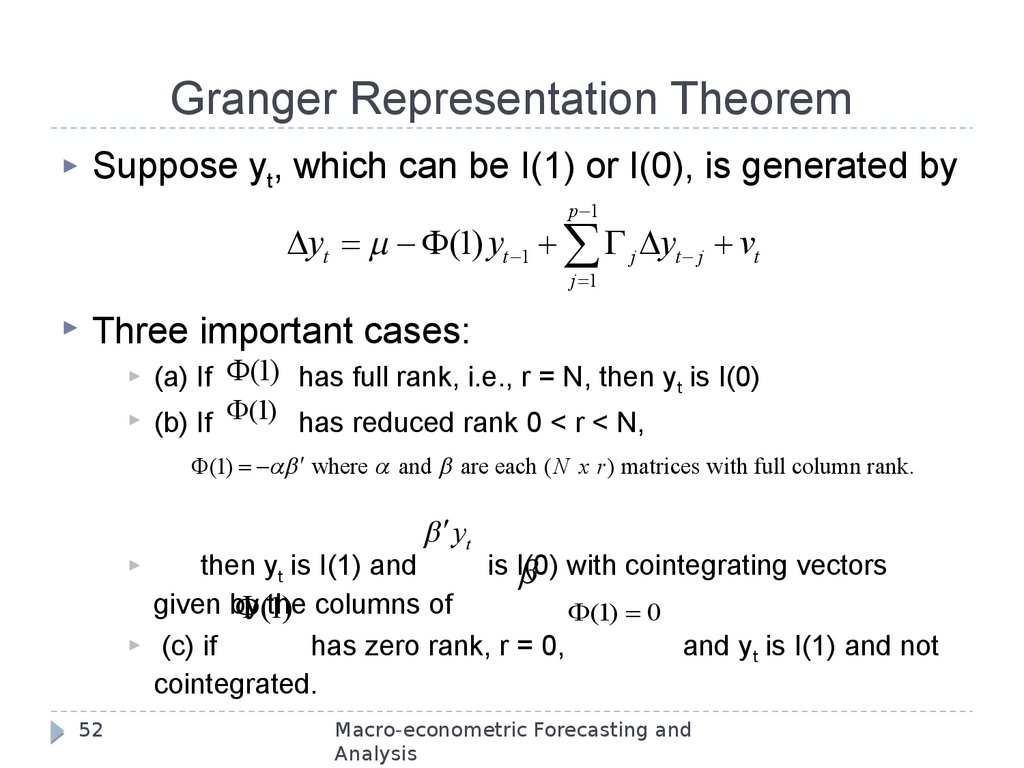
Granger Representation Theorem
Suppose yt, which can be I(1) or I(0), is generated by
p 1
yt F (1) yt 1 G j yt j vt
j 1
Three important cases:
(a) If F (1) has full rank, i.e., r = N, then yt is I(0)
(b) If F (1) has reduced rank 0 < r < N,
F (1) ab ¢ where a and b are each ( N x r ) matrices with full column rank.
b ¢ yt
52
then yt is I(1) and
is I(0)
b with cointegrating vectors
given by
the columns of
F (1)
F (1) 0
(c) if
has zero rank, r = 0,
and yt is I(1) and not
cointegrated.
Macro-econometric Forecasting and
Analysis

53. Examples: Rank of Long-Run Models

The form of F (1) for the two long-run models we
considered above:
Permanent Income: (N=2, r=1)
Term structure: (N = 3, r = 2)
éa1,1 ù é 1 ù¢
F (1) ab ¢ ê ú ê
ú
b
a
ë 2,1 û ë y û
éa1,1 a1,2 ù é 1 0 ù¢
ê
ú
ê
ú
F (1) ab ¢ êa 2,1 a 2,2 ú ê 0 1 ú
êëa 3,1 a 3,2 úû êë b 3,1 b3,2 úû
53
Macro-econometric Forecasting and
Analysis

54.

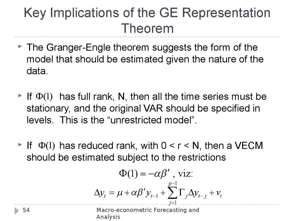
Key Implications of the GE Representation
Theorem
The Granger-Engle theorem suggests the form of the
model that should be estimated given the nature of the
data.
If F (1) has full rank, N, then all the time series must be
stationary, and the original VAR should be specified in
levels. This is the “unrestricted model”.
If F (1) has reduced rank, with 0 < r < N, then a VECM
should be estimated subject to the restrictions
F (1) ab ¢ , viz:
p 1
yt ab ¢ yt 1 G j yt j vt
54
j 1
Macro-econometric Forecasting and
Analysis

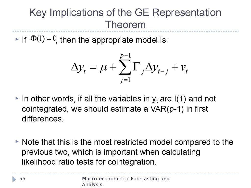
55.

Key Implications of the GE Representation
Theorem
If F (1) 0, then the appropriate model is:
p 1
yt G j yt j vt
j 1
In other words, if all the variables in yt are I(1) and not
cointegrated, we should estimate a VAR(p-1) in first
differences.
Note that this is the most restricted model compared to the
previous two, which is important when calculating
likelihood ratio tests for cointegration.
55
Macro-econometric Forecasting and
Analysis

56. Dealing With Deterministic Components

We can easily extend the base VECM to include a
deterministic time trend, viz:
p 1
yt 0 1t ab ¢ yt 1 G j yt j vt
j 1
where now 0 and 1 are (N x 1) vectors of
parameters associated with the intercept and time
trend.
The deterministic components can contribute both to
the short-run and the long-run components of y t
56
Macro-econometric Forecasting and
Analysis

57. Deterministic Components

Suppose we can decompose these parameters into
their short-run and long-run components by defining:
j j ab ¢j , j 0, 1
where j (N x 1) is the short-run component and ab ¢j
is the long-run component.
We can rewrite the model as:
p 1
yt 0 1t a ( b 0¢ b1¢t b ¢ yt 1 ) G j yt j vt
j 1
57
Macro-econometric Forecasting and
Analysis

58. Deterministic Components

The term ( b 0¢ b1¢t b ¢ yt 1 ) represents the long-run
relationship among the variables.
The parameter 0 provides a drift component in the
equation of yt , so it contributes a trend to yt
Similarly 1t allows for linear time trend in yt and a
quadratic trend to yt
By contrast, b 0 contributes a constant to the EC-Eq
b1¢t
and
contributes a linear time trend to EC-Eq
58
Macro-econometric Forecasting and
Analysis

59. Deterministic Components

The equation
p 1
yt 0 1t a ( b 0¢ b1¢t b ¢ yt 1 ) G j yt j vt
j 1
contains five important special cases summarized on the next
slide.
Model 1 is the simplest (and most restricted) as there are no
deterministic components.
Model 2 allows for r intercepts in the long-run equations.
Model 3 (most common) allows for constants in both the shortrun and the long-run equations – total of N+r intercepts.
59
Macro-econometric Forecasting and
Analysis

60. Alternative Deterministic Structures

60
Macro-econometric Forecasting and
Analysis

61. Estimating VECM Models

If you are willing to assume that the error term vt is
white noise and N(0,σ2), the parameters of the VECM
can be estimated directly by full-information maximum
likelihood techniques.
Basically, one estimates a traditional VAR subject to the
cross-equation restrictions implied by cointegration.
Using FIML is the most flexible approach, but it requires
one to ensure that the parameters of the overall model
are identified (via exclusion restrictions). More on this
later.
61
Macro-econometric Forecasting and
Analysis

62. Three Cases:

F (1) can be inverted.
VECM is equivalent to the unconstrained VAR. No
restrictions are imposed on the VAR.
Maximum likelihood estimator is obtained by
applying OLS to each equation separately.
The estimator is applied to the levels of the data,
since they are (must be) stationary.
62
Macro-econometric Forecasting and
Analysis

63. Reduced Rank (Cointegration) Case: FIML

If F (1) cannot be inverted (i.e., reduced rank case, or
we are dealing with a cointegrated system), we
impose the cross-equation restrictions coming from
the lagged ECM term(s), and then estimate the
system using full-information maximum likelihood
methods.
The VECM is a restricted model compared to the
unconstrained VAR.
63
Macro-econometric Forecasting and
Analysis

64. Reduced Rank Case: Johansen Estimator

We can also use the Johansen (1988) estimator.
This differs from FIML in that the cross-equation
identifying restrictions are NOT imposed on the
model before estimation.
The Johansen approach estimates a basis for the
vector space spanned by the cointegrating vectors,
and THEN imposes identification on the coefficients.
64
Macro-econometric Forecasting and
Analysis

65. Zero-Rank Case for

F(1)
When F (1) 0, the VECM reduces to a VAR in
first differences.
As with the full-rank model, the maximum
likelihood estimator is the ordinary least squares
estimator applied to each equation separately.
This is the most constrained model compared to
a VECM/unconstrained VAR in levels.
65
Macro-econometric Forecasting and
Analysis

66. Identification

The Johansen procedure requires one to normalize
the cointegrating vectors so that one of the variables
in the equation is regarded as the dependent
variable of the long-run relationship.
In the bi-variate term structure and the permanent
income example, the normalization takes the form of
designating one of variables in the system as the
dependent variable.
66
Macro-econometric Forecasting and
Analysis

67. Identification: Triangular Restrictions

Suppose there are r long-run relationships.
Identification can be achieved by transforming the
top (r x r) block of bˆ (the long-run parameters) to
the identity matrix.
If r = 1, this corresponds to normalizing one the
coefficients to unity.
67
Macro-econometric Forecasting and
Analysis

68. Triangular Restrictions

If there are N = 3 variables and r = 2 cointegrating
equations, one sets bˆ to:
é 1 0 ù
ê
ú
ˆ
b ê 0 1 ú
êˆ
ú
ˆ
ë b 3,1 b3,2 û
This form of the normalized estimated co-integrated
vector is appropriate for the tri-variate term structure
model introduced earlier.
68
Macro-econometric Forecasting and
Analysis

69. Structural Restrictions

Traditional identification methods can also be used
with VECM’s, including exclusion restrictions, crossequation restrictions, and restrictions on the
disturbance covariance matrix.
Example: Johansen and Juselius(1992) propose an
open economy model in which yt { st , pt , pt* , it , it*}
represents, respectively, the spot exchange rate, the
domestic price level, the foreign price, the domestic
interest rate and the foreign interest rate.
Thus, N = 5.
69
Macro-econometric Forecasting and
Analysis

70. Open Economy Model

Assuming r = 2 long-run equations, the following
restrictions consisting of normalization, exclusion
and cross-equation restrictions on yield the
normalized long-run parameter matrix
é1 b 2,1 b 2,1 0 0 ù
b¢ ê
ú
b
ë0 0 0 1 5,1 û
The long-run equations represent PPP and UIP.
st b 2,1 ( pt pt* ) u1,t [PPP]
it b 5,1it* u2,t
70
[Uncovered IP]
Macro-econometric Forecasting and
Analysis

71. Cointegration Rank

So far we have taken the rank of the system as given. But
how do we decide how many co-integrating vectors are in
the vector of N variables?
Simple approach is to estimate models of different rank and
then do a formal likelihood ratio test to decide whether
restricted model (i.e., the model with rank r less than N) is
appropriate.
Specifically, one would estimate the most restricted model (r
= 0), a model that assumes (r=1), then a model that
assumes r = 2, etc. The process ends when we cannot
reject the null (r = r0).
71
Macro-econometric Forecasting and
Analysis

72. Cointegration Rank: Likelihood Ratio Test

Suppose we estimate the model assuming no
cointegration. Let the parameters involved in that
model be denoted byqˆr N .
Let the value of the likelihood of this model be
denoted by LT qˆr N
Now estimate the model assuming r ≥ 1. Obviously,
this is an restricted model compared to the r = N
case. Let the value of the likelihood in this case be
denoted by LT qˆr r
(
)
(
72
0
)
Macro-econometric Forecasting and
Analysis

73. Cointegration Rank: Likelihood Ratio Test

Using the standard result for the likelihood ratio test,
we get the following LR test statistic:
(
(
)
(
LR 2 (T p) ln LT qˆr r0 (T p ) ln LT qˆr N
))
We reject the restricted model if the likelihood ratio
test is greater than the corresponding critical value.
In this case, imposing the restrictions does not yield a
superior model.
73
Macro-econometric Forecasting and
Analysis

74. Cointegration Rank: Johansen Approach

A numerically equivalent approach was proposed by
Johansen (1988).
He expressed the problem in terms of the eigen values
of the likelihood function – an approach that is
numerically equivalent to the likelihood ratio test. He
termed it the “trace statistic”.
The critical values of the LR test are non-standard, and
depend on the structure of the deterministic part of the
model. Critical values are shown on the next slide.
74
Macro-econometric Forecasting and
Analysis

75. Critical Values of the Likelihood Ratio Test

75
Macro-econometric Forecasting and
Analysis

76. Tests on the Cointegrating Vector (Long-Run Parameters)

b
Hypothesis tests on the cointegrating vector, ,
constitute tests of long-run economic theories.
In contrast to the cointegration rank tests, the
asymptotic distribution of the Wald, Likelihood Ratio
2
c
and Lagrange Multiplier tests
is under the null
hypothesis that the restrictions are valid.
76
Macro-econometric Forecasting and
Analysis

77. Exogeneity

An important feature of a VECM is that all of the variables
in the system are endogenous.
When the system is out of equilibrium, all the variables
interact with each other to move the system back into
equilibrium,
In a VECM, this process occurs (as we saw) through the
impact of lagged variables so that yi,t is affected by the
lags of the other variables either through the error
correction term, ut-1, or through the lags of y j ,t , j ¹ i
77
Macro-econometric Forecasting and
Analysis

78. Weak versus Strong Exogeneity

If the first channel does not exist, i.e., the lagged error
correction term does not influence the adjustment
process, the variable concerned is said to be weakly
exogenous.
If the first and second channels do not exist, then only
the lagged values of a variable can be used to explain
its changes. In this case, we say that that variable is
strongly exogenous.
Strong exogeneity testing is equivalent to Granger
causality testing.
78
Macro-econometric Forecasting and
Analysis

79. Example: Exogeneity

Consider the bi-variate term structure model with
one cointegrating vector.
y a1 ( y
10
t
10
t 1
p 1
p 1
b 0 b y ) 10,i y 10,i yt1 i t
1
1 t 1
i 1
10
t i
i 1
p 1
p 1
i 1
i 1
yt1 a 2 ( yt10 1 b 0 b1 yt1 1 ) 1,i yt10 i 1,i yt1 i t
10
y
The ten-year interest rate, t , is said to be weakly
exogenous if a1 0
Strong exogeneity amounts to the requirement that
a1 0, 10,i 0 i
79
Macro-econometric Forecasting and
Analysis

80. Impulse Response Functions

The dynamics of a VECM can be investigated using
impulse response functions.
The approach is to re-express the VECM as a VAR,
but preserving the implied restrictions on the
parameters.
For example, consider the VECM
p 1
yt 0 1t ab ¢ yt 1 G j yt j vt
j 1
80
Macro-econometric Forecasting and
Analysis

81. Impulse Response Functions: VECM

This VECM can be expressed as a VAR in levels:
p
yt F j yt j vt
j 1
subject to the restrictions:
F1 ab ¢ G1 I N
F j G j G j 1 , j 2,3,L , p
81
Macro-econometric Forecasting and
Analysis

82. Appendices

83. Appendix A: Process moments, key results: AR(1) model with θ < 1

Appendix A: Process moments, key results:
AR(1) model with θ < 1
Mean (first moment):
(8)
t 1
j 0
j 0
as t
1 q
Variance (second moment):
(9)
t 1
E[ yt ] q q j vt j q t y0
j
é t 1 j
2ù
2
var[ yt ] E[( yt E[ yt ]) ] E ê ( q vt j ) ú
as t
2
ë j 0
û 1 q
2
Key point to note is that the first and second moments are converging to finite
constants.
1 T
1 T 2
p
p
yt 1 ¾¾
lim E [ yt ] and yt 1 ¾¾
lim E éë yt2 ùû
t
t
T t 2
T t 2
So WLLN applies:
So any estimator based on these quantities should converge in a similar fashion.
83
Macro-econometric Forecasting and
Analysis

84. Appendix A: Process moments, Simulation of an AR(1) model

Assume
0.0, 0.8, 2 1.0
It follows that
lim E [ yt ]
t
0.0
0.0
1 q 1 0.8
2
1.0
lim var(yt )
2.778
t
1 q 2 1 0.82
Also
Note that the sample moments converge to these values as the sample size
increases. Also, the variance of the estimator is approaching zero as T
increases.
84
Macro-econometric Forecasting and
Analysis

85. Appendix A: Process moments, key results: AR(1) model with θ = 1

First moment:
t 1
E [ yt ] q y0 q j y0 t
t
j 0
Second moment:
var( yt )
2
t 1
2j
2
2
4
2
q
(1
q
q
K
)
t
j 0
Appropriate scaling factors for these moments are T 3/2
2
T
and
respectively.
Define
85
m1
1
T 3/2
T
1
yt 1 , m2 2
T
t 2
T
2
y
t 1
t 2
(sample moments)
Macro-econometric Forecasting and
Analysis

86. Appendix A: Process moments, simulation of an I(1) Process

Notice that the variances of the first two sample moments do not fall
as the sample size is increased (Columns 2 and 4).
The variances converge to 1/3, so m1 and m2 converge to random
variables in the limit.
86
Macro-econometric Forecasting and
Analysis

87. Appendix B: Enders Strategy

Estimate yt = 1+ 2t+ yt-1 + εt
No unit root (yt is stationary). Additional
testing is needed for deterministic
components
Test H0: =0
t-ratio test, 5% Crit. value is
-3.45
Test H0: 2= =0
F-test, 5% Crit. value is
6.49
Estimate yt = 1+ yt-1 + εt
Test H0: =0
t-ratio test, 5% Crit. value is
-2.89
Test H0: 1= =0
F-test, 5% Crit. value is
4.71
Estimate yt = yt-1
+ εt
Test H0: =0
t-ratio test, 5% Crit. value is -1.64
Test H0: =0 using Ndistribution
t-test, 5% Crit. value isNo
-1.64
unit root (yt is
Unit root (yt has both
stationary around
stochastic and
deterministic trend).
deterministic trends).
yt = 1+ 2t+θyt-1 + εt ,|
yt = 1+ 2t + yt-1 + εt
No unit root (yt is
θ|<1
stationary). Additional
testing of 1 is needed
Test H0: =0 using Ndistribution
t-test, 5% Crit. value is -1.64
No unit root (yt is
Unit root (yt is nonstationary).
stationary) yt = 1+yt-1 + εt
yt = 1+θyt-1 + εt ,|θ|<1
No unit root (yt is
stationary).
yt = θyt-1 + εt ,|θ|<1
Unit root (yt is non-stationary). yt = yt-1 +
εt
87

88. Appendix B: Enders Strategy (2)

Enders Strategy was criticized for:
triple- and double-testing for unit roots
unrealistic outcomes: economic variables unlikely contain both
stochastic and deterministic trend as in
yt = 1+ 2t+ yt-1 + εt , 2≠0, =0,
this possibility should be excluded from the test
not taking advantage of prior knowledge
Alternative: Elder and Kennedy Strategy
88

89. Appendix B: Elder and Kennedy Strategy

Estimate yt = 1+ 2t+ yt-1 + εt
Test H0: =0
t-ratio test, 5% Crit. value is
-3.45
Unit root (yt is nonstationary).
Estimate yt = 1+ εt
Test H0: 1=0
double sided t-test,
5% Crit. values are
-1.95<t<1.95
Unit root (yt is nonstationary without
intercept):
yt = yt-1 + εt
No unit root (yt is stationary).
Test H0: 2=0
double sided t-test,
5% Crit. values are
-1.95<t<1.95
No unit root (yt is
No unit root (yt is
stationary around
stationary without
deterministic trend).
deterministic trend):
yt = 1+ 2t+θyt-1 + εt ,|θ|
yt = 1+ θyt-1 + εt ,|θ|<1
<1
Unit root (yt is nonstationary with intercept).
yt = 1+ yt-1 + εt
89

90. Nonstationary Asymptotics

90
Macro-econometric Forecasting and
Analysis

91. Nonstationary Asymptotics

Source: faculty.washington.edu/ezivot/econ584/notes/unitroot.pdf
91
Macro-econometric Forecasting and
Analysis