Good morning! Доброе утро! 早上好! Machine learning lecture 3

1. Good morning! Доброе утро! 早上好!

Lecture2. Data Structures in Python for Data analysis
Good morning!
Доброе утро!
早上好!

2. 我们会成功

Lecture2. Data Structures in Python for Machine learning
我们会成功
We will succeed !
У нас все получится [U nas vse poluchitsya ] !
Без булдырабыз!

3. .

Lecture3.
Data
preproccessing
and
.
machine learning with Scikitlearn

4.

Извлечение признаков и масшатбирование,
будущая выборка, уменьшение размерности
выборки

5. Training set and testing set

• Machine learning is about learning some properties of a data set and
then testing those properties against another data set.
• A common practice in machine learning is to evaluate an algorithm
by splitting a data set into two.
• We call one of those sets the training set, on which we learn some
properties; we call the other set the testing set, on which we test the
learned properties.

6. Reading a Dataset

7.

8. Data Description :

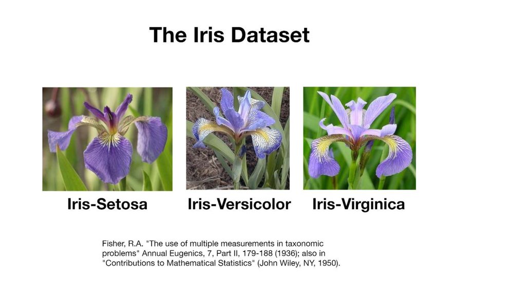
Attribute Information:
1. sepal length in cm
2. sepal width in cm
3. petal length in cm
4. petal width in cm
Class:
-- Iris Setosa
-- Iris Versicolour
-- Iris Virginica

9.

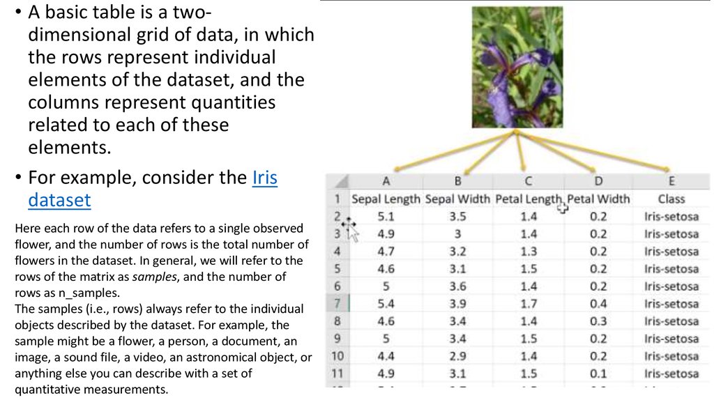
• A basic table is a twodimensional grid of data, in which
the rows represent individual
elements of the dataset, and the
columns represent quantities
related to each of these
elements.
• For example, consider the Iris
dataset
Here each row of the data refers to a single observed
flower, and the number of rows is the total number of
flowers in the dataset. In general, we will refer to the
rows of the matrix as samples, and the number of
rows as n_samples.
The samples (i.e., rows) always refer to the individual
objects described by the dataset. For example, the
sample might be a flower, a person, a document, an
image, a sound file, a video, an astronomical object, or
anything else you can describe with a set of
quantitative measurements.

10. Target array

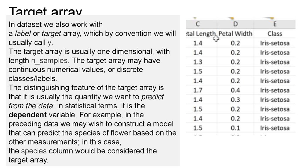
In dataset we also work with
a label or target array, which by convention we will
usually call y.
The target array is usually one dimensional, with
length n_samples. The target array may have
continuous numerical values, or discrete
classes/labels.
The distinguishing feature of the target array is
that it is usually the quantity we want to predict
from the data: in statistical terms, it is the
dependent variable. For example, in the
preceding data we may wish to construct a model
that can predict the species of flower based on the
other measurements; in this case,
the species column would be considered the
target array.

11.

• Basic Data Analysis :
• The dataset provided has 150 rows
• Dependent Variables : Sepal length.Sepal Width,Petal length,Petal
Width
• Independent/Target Variable : Class
• Missing values : None

12.

•The dataset is divided into
Train and Test data
with 80:20 split ratio
where 80% data is training data where as
20% data is test data.

13.

• Each training point belongs to one of N different
classes.
• The goal is to construct a function which, given a
new data point, will correctly predict the class to
which the new point belongs.
Classification: samples belong to two or more
classes and we want to learn from already labeled
data how to predict the class of unlabeled data.

14. What is scikit-learn?

The scikit-learn library provides an
implementation of a range of algorithms for
Supervised Learning and Unsupervised Learning.

15. You can watch the Pandas and scikit-learn features documentation on this site.

• https://pandas.pydata.org/pandas-docs/stable/
https://scikit-learn.org/stable/documentation.html

16. Preprocessing Data: missing data

• Real world data is filled with missing values.
• You will often need to rid your data of these missing values in order to
train a model or do meaningful analysis.
• What follows are a few ways to impute (fill) missing values in Python,
for both numeric and categorical data.

17.

18.

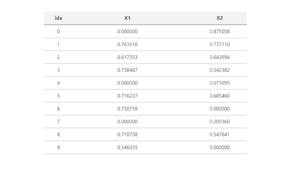
Method 1: Mean or Median
• A common method of imputation with numeric features is to replace
missing values with the mean of the feature’s non-missing values. If
the data have outliers, you may want to use the median instead.
Either method is easy in Pandas:
df_mean_imputed = df.fillna(df.mean())
df_median_imputed = df.fillna(df.median())

19.

20. Imputation Method 2: Zero

• Depending on where your data are coming from, a missing value may
be better represented by the number zero. Replacing missing values
with zeros is accomplished similar to the above method; just replace
the mean function with zero.

21.

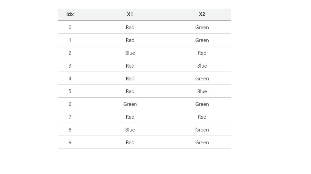
22. Imputation for Categorical Data

• For categorical features, using mean, median, or
zero-imputation doesn’t make much sense. Here
I’ll create an example dataset with categorical
features and show two imputation methods
specific to this type of data.

23.

24. Imputation Method 1: Most Common Class

• One approach to imputing categorical features is to replace missing
values with the most common class. You can do with by taking the
index of the most common feature given in Pandas’ value_counts
function.
# for each column, get value counts in decreasing order and take the index (value) of most
common class
df_most_common_imputed = colors.apply(lambda x: x.fillna(x.value_counts().index[0]))

25.

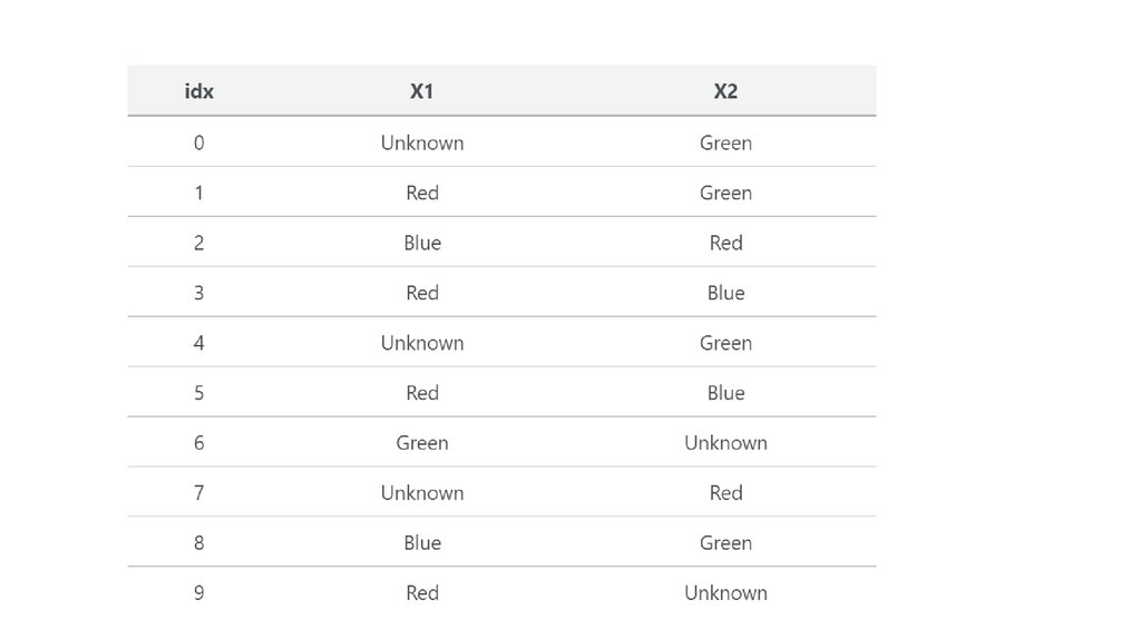
26. Imputation Method 2: “Unknown” Class

• Similar to how it’s sometimes most appropriate to impute a missing
numeric feature with zeros, sometimes a categorical feature’s
missing-ness itself is valuable information that should be explicitly
encoded. If this is the case, most-common-class imputing would
cause this information to be lost. Instead, just replace those values
with a value like “Unknown” or “Missing.”
• df_unknown_imputed = colors.fillna("Unknown")

27.

28. Column-Specific Imputation Rules

• You can combine any of the above methods by imputing specific
columns rather than the entire dataframe. Returning to the numeric
example, we can mean-impute X1 and median-impute X2 by
specifying the column(s) to be imputed.
• # replace missing values with the column mean

29. Preprocessing Data If data set are strings

• We saw in our initial exploration that most of the columns in our data
set are strings, but the algorithms in scikit-learn understand only
numeric data. Luckily, the scikit-learn library provides us with many
methods for converting string data into numerical data. One such
method is the LabelEncoder() method. We will use this method to
convert the categorical labels in our data set like ‘won’ and ‘loss’ into
numerical labels. To visualize what we are trying to to achieve with
the LabelEncoder() method let’s consider the images below.

30.

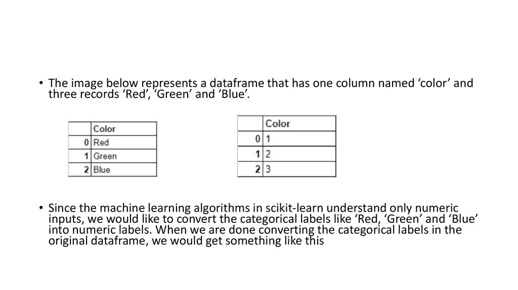
• The image below represents a dataframe that has one column named ‘color’ and
three records ‘Red’, ‘Green’ and ‘Blue’.
• Since the machine learning algorithms in scikit-learn understand only numeric
inputs, we would like to convert the categorical labels like ‘Red, ‘Green’ and ‘Blue’
into numeric labels. When we are done converting the categorical labels in the
original dataframe, we would get something like this

31.

#import the necessary module
from sklearn import preprocessing
# create the Labelencoder object
le = preprocessing.LabelEncoder()
#convert the categorical columns into numeric
encoded_value = le.fit_transform(["paris", "paris", "tokyo", "amsterdam"])
print(encoded_value)
he LabelEncoder() method assigns the numeric values to the classes in the order of the first letter of
the classes from the original list: “(a)msterdam” gets an encoding of ‘0’ , “(p)aris gets an encoding of 1”
and “(t)okyo” gets an encoding of 2.

32. Training Set & Test Set

Training Set & Test Set
• A Machine Learning algorithm needs to be trained on a set of data to
learn the relationships between different features and how these
features affect the target variable.
• For this we need to divide the entire data set into two sets.
• One is the training set on which we are going to train our algorithm to
build a model.
• The other is the testing set on which we will test our model to see
how accurate its predictions are.

33.

But before doing all this splitting, let’s first separate our features and
target variables.
#import the necessary module
from sklearn.model_selection import train_test_split
#split data set into train and test setsdata_train, data_test,
target_train, target_test = train_test_split(data, target, test_size = 0.30)
we used the train_test_split() method to divide the data into a training set (data_train,target_train) and a test set
(data_test,data_train). The first argument of the train_test_split() method are the features that we separated out in the
previous section, the second argument is the target(‘Opportunity Result’). The third argument ‘test_size’ is the
percentage of the data that we want to separate out as training data .

34. Watch subtitled video

• https://www.coursera.org/lecture/machine-learning/what-ismachine-learning-Ujm7v

35.

36.

37. CHECK