Похожие презентации:
The Inverted Multi-Index
1. The Inverted Multi-Index
Victor Lempitskyjoint work with
Artem Babenko
VGG Oxford, 25 Oct 2012
1/26
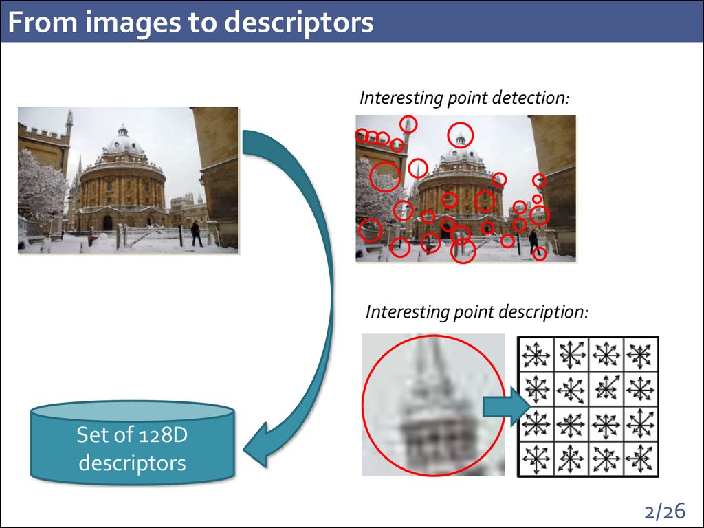
2. From images to descriptors
Interesting point detection:Interesting point description:
Set of 128D
descriptors
2/26
3. Query process
Image set:Dataset of visual
descriptors
Main operation:
Finding similar descriptors
Important extras:
+ geometric verification
+ query expansion
Query:
3/26
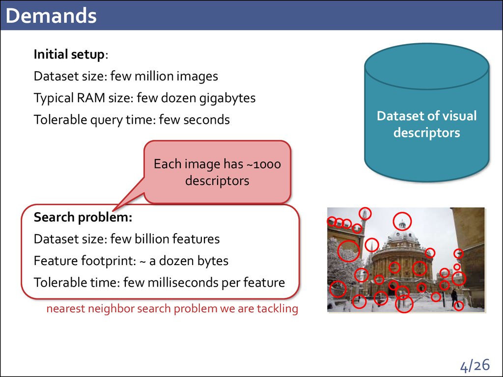
4. Demands
Initial setup:Dataset size: few million images
Typical RAM size: few dozen gigabytes
Tolerable query time: few seconds
Dataset of visual
descriptors
Each image has ~1000
descriptors
Search problem:
Dataset size: few billion features
Feature footprint: ~ a dozen bytes
Tolerable time: few milliseconds per feature
nearest neighbor search problem we are tackling
4/26
5. Meeting the demands
Main observation: the vectors have a specific structure:correlated dimensions, natural image statistics, etc…
Technologies:
• Dimensionality reduction
Our contribution:
• Vector quantization
Inverted Multi-Index
• Inverted index
• Locality-sensitive hashing
• Product quantization
• Binary/Hamming encodings
Best combinations (previous state-of-the-art):
• Inverted index + Product Quantization [Jegou et al. TPAMI 2011]
• Inverted index + Binary encoding [Jegou et al. ECCV 2008]
New state-of-the-art for BIGANN:
• Inverted multi-index + Product Quantization [CVPR 2012]
5/26
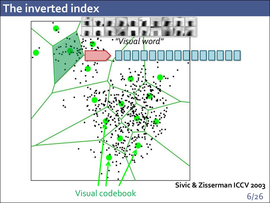
6. The inverted index
"Visual word"Sivic & Zisserman ICCV 2003
Visual codebook
6/26
7. Querying the inverted index
Query:• Have to consider
several words for best
accuracy
• Want to use as big
codebook as possible
conflict
• Want to spend as little
time as possible for
matching to codebooks
7/26
8. Product quantization
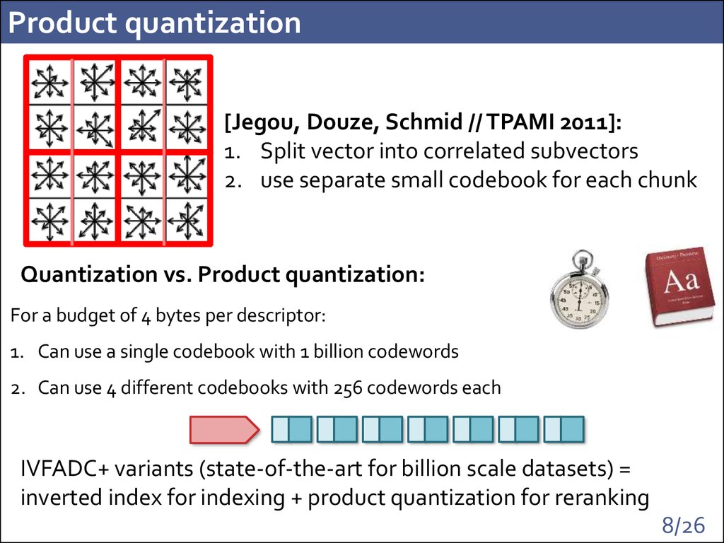
[Jegou, Douze, Schmid // TPAMI 2011]:1. Split vector into correlated subvectors
2. use separate small codebook for each chunk
Quantization vs. Product quantization:
For a budget of 4 bytes per descriptor:
1. Can use a single codebook with 1 billion codewords
many minutes
128GB
2. Can use 4 different codebooks with 256 codewords each < 1 millisecond 32KB
IVFADC+ variants (state-of-the-art for billion scale datasets) =
inverted index for indexing + product quantization for reranking
8/26
9. The inverted multi-index
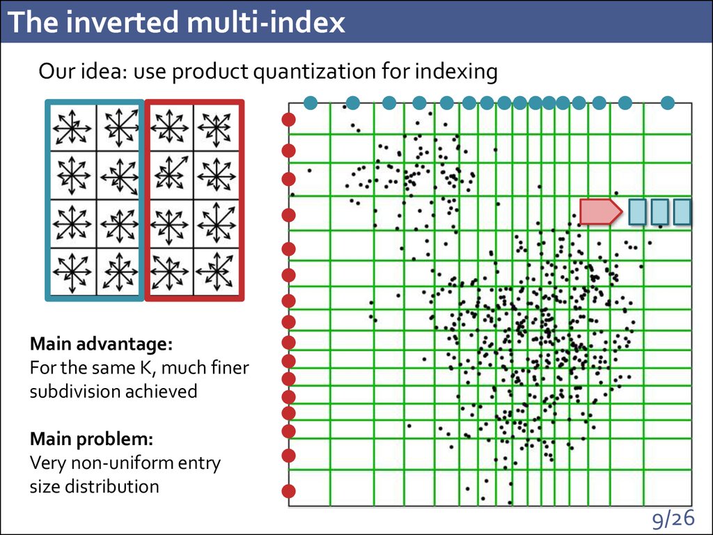
Our idea: use product quantization for indexingMain advantage:
For the same K, much finer
subdivision achieved
Main problem:
Very non-uniform entry
size distribution
9/26
10. Querying the inverted multi-index
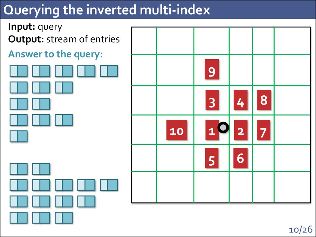
Input: queryOutput: stream of entries
Answer to the query:
9
10
3
4
8
1
2
7
5
6
10/26
11. Querying the inverted multi-index – Step 1
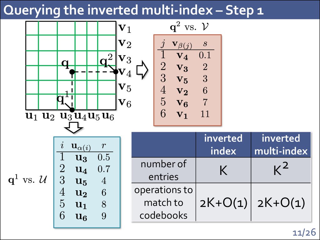
number ofentries
operations to
match to
codebooks
inverted
index
inverted
multi-index
K
2
K
2K+O(1) 2K+O(1)
11/26
12. Querying the inverted multi-index – Step 2
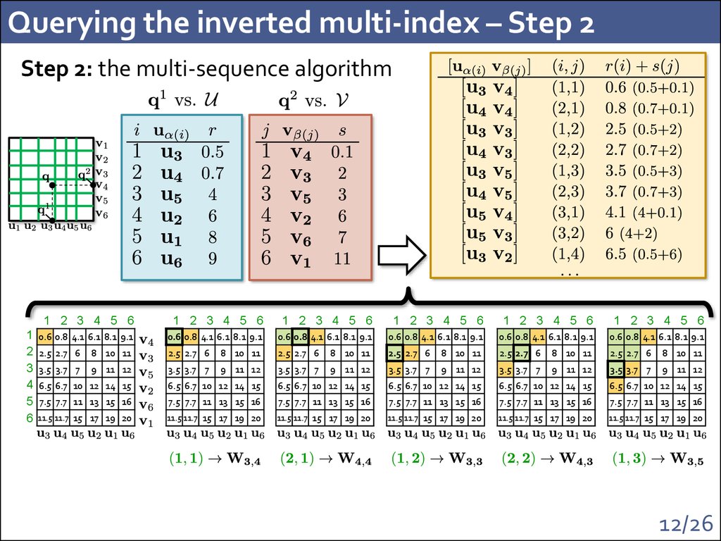
Step 2: the multi-sequence algorithm1
2
3
4
5
6
1 2 3 4 5 6
1 2 3 4 5 6
1 2 3 4 5 6
1 2 3 4 5 6
1 2 3 4 5 6
1 2 3 4 5 6
0.6 0.8 4.1 6.1 8.1 9.1
0.6 0.8 4.1 6.1 8.1 9.1
0.6 0.8 4.1 6.1 8.1 9.1
0.6 0.8 4.1 6.1 8.1 9.1
0.6 0.8 4.1 6.1 8.1 9.1
0.6 0.8 4.1 6.1 8.1 9.1
2.5 2.7 6
8 10 11
2.5 2.7 6
8 10 11
2.5 2.7 6
8 10 11
2.5 2.7 6
8 10 11
2.5 2.7 6
8 10 11
2.5 2.7 6
8 10 11
3.5 3.7 7
9 11 12
3.5 3.7 7
9 11 12
3.5 3.7 7
9 11 12
3.5 3.7 7
9 11 12
3.5 3.7 7
9 11 12
3.5 3.7 7
9 11 12
6.5 6.7 10 12 14 15
6.5 6.7 10 12 14 15
6.5 6.7 10 12 14 15
6.5 6.7 10 12 14 15
6.5 6.7 10 12 14 15
6.5 6.7 10 12 14 15
7.5 7.7 11 13 15 16
7.5 7.7 11 13 15 16
7.5 7.7 11 13 15 16
7.5 7.7 11 13 15 16
7.5 7.7 11 13 15 16
7.5 7.7 11 13 15 16
11.5 11.7 15 17 19 20
11.5 11.7 15 17 19 20
11.5 11.7 15 17 19 20
11.5 11.7 15 17 19 20
11.5 11.7 15 17 19 20
11.5 11.7 15 17 19 20
12/26
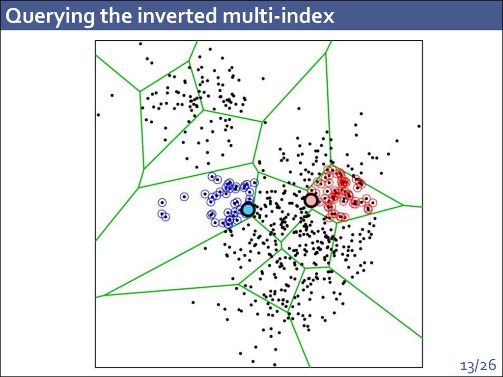
13. Querying the inverted multi-index
13/2614. Experimental protocol
Dataset:1. 1 billion of SIFT vectors [Jegou et al.]
2. Hold-out set of 10000 queries, for which Euclidean nearest neighbors are known
Comparing index and multi-index:
Set a candidate set length T
For each query:
• Retrieve closest entries from index or multi-index and concatenate lists
• Stop when the next entry does not fit
For small T inverted index can return empty list
• Check whether the true neighbor is in the list
Report the share of queries where the neighbor was present (recall@T)
14/26
15. Performance comparison
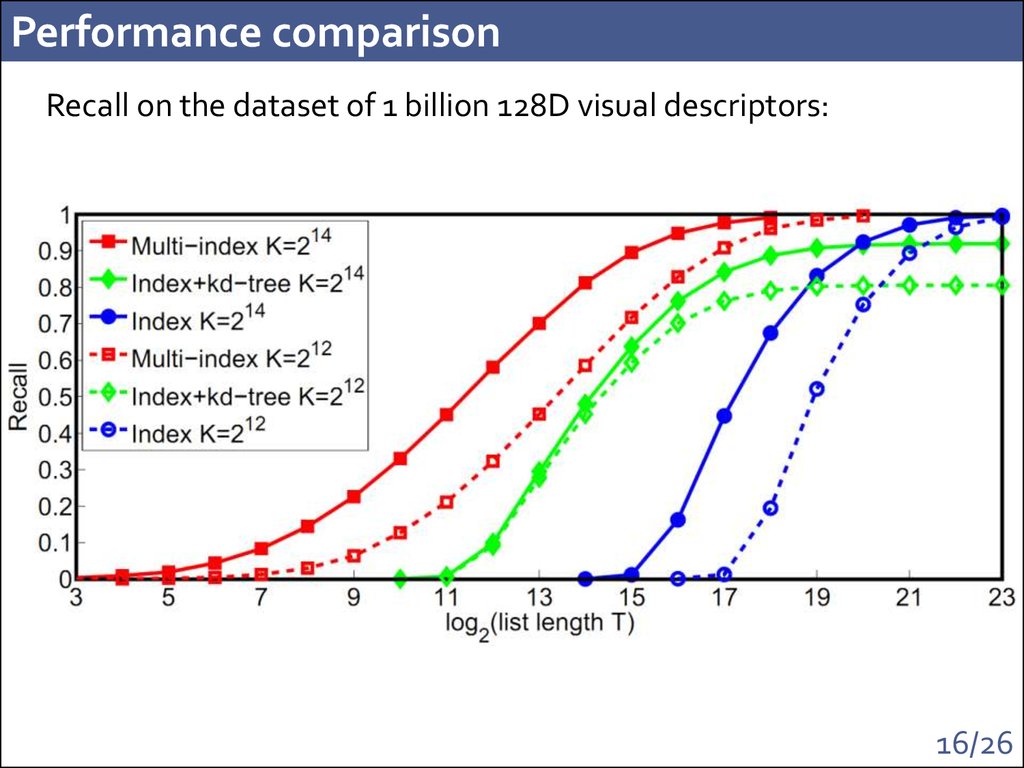
Recall on the dataset of 1 billion of visual descriptors:"How fast can we catch the nearest neighbor to the query?"
100x
K = 214
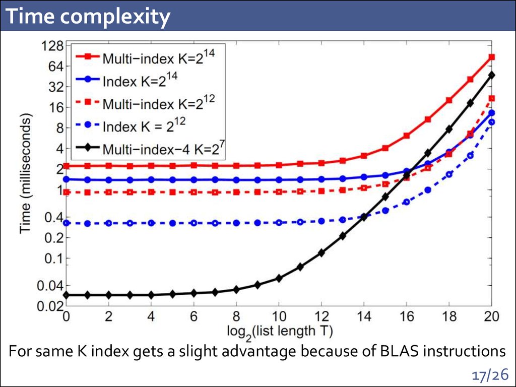
Time increase: 1.4 msec -> 2.2 msec on a single core
(with BLAS instructions)
15/26
16. Performance comparison
Recall on the dataset of 1 billion 128D visual descriptors:16/26
17. Time complexity
For same K index gets a slight advantage because of BLAS instructions17/26
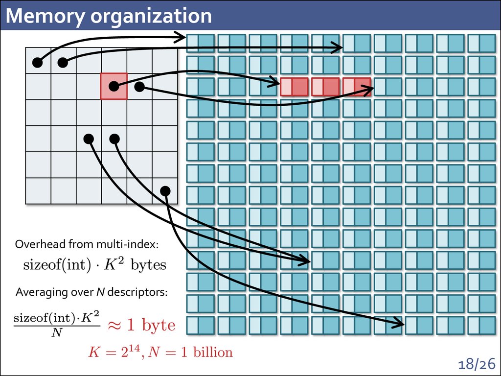
18. Memory organization
Overhead from multi-index:Averaging over N descriptors:
18/26
19. Why two?
For larger number of parts:• Memory overhead becomes larger
• Population densities become even more non-uniform
(multi-sequence algorithm has to work harder to
accumulate the candidates)
In our experiments, 4 parts with small K=128 may be competitive
for some datasets and reasonably short candidate lists (e.g.
duplicate search). Indexing is blazingly fast in these cases!
19/26
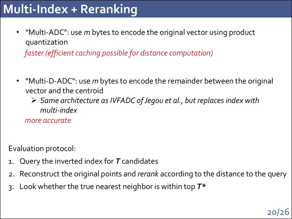
20. Multi-Index + Reranking
• "Multi-ADC": use m bytes to encode the original vector using productquantization
faster (efficient caching possible for distance computation)
• "Multi-D-ADC": use m bytes to encode the remainder between the original
vector and the centroid
Same architecture as IVFADC of Jegou et al., but replaces index with
multi-index
more accurate
Evaluation protocol:
1. Query the inverted index for T candidates
2. Reconstruct the original points and rerank according to the distance to the query
3. Look whether the true nearest neighbor is within top T*
20/26
21. Multi-ADC vs. Exhaustive search
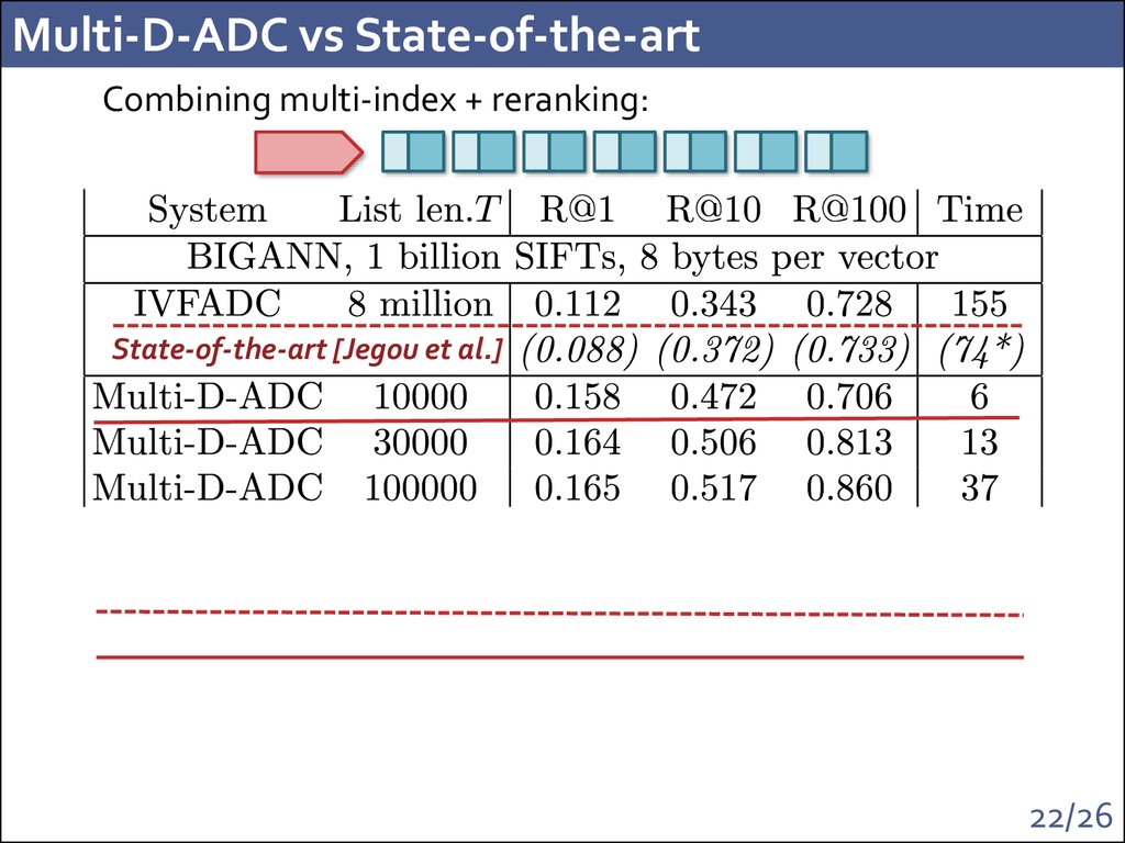
21/2622. Multi-D-ADC vs State-of-the-art
Combining multi-index + reranking:State-of-the-art [Jegou et al.]
22/26
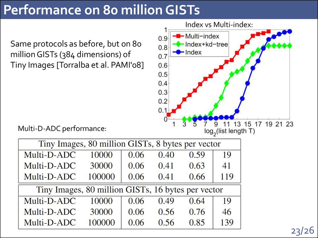
23. Performance on 80 million GISTs
Index vs Multi-index:Same protocols as before, but on 80
million GISTs (384 dimensions) of
Tiny Images [Torralba et al. PAMI'08]
Multi-D-ADC performance:
23/26
24. Retrieval examples
Exact NNUncompressed GIST
Multi-D-ADC
16 bytes
Exact NN
Uncompressed GIST
Multi-D-ADC
16 bytes
Exact NN
Uncompressed GIST
Multi-D-ADC
16 bytes
Exact NN
Uncompressed GIST
Multi-D-ADC
16 bytes
24/26
25. Multi-Index and PCA (128->32 dimensions)
Multi-Index and PCA (128->32 dimensions)25/26
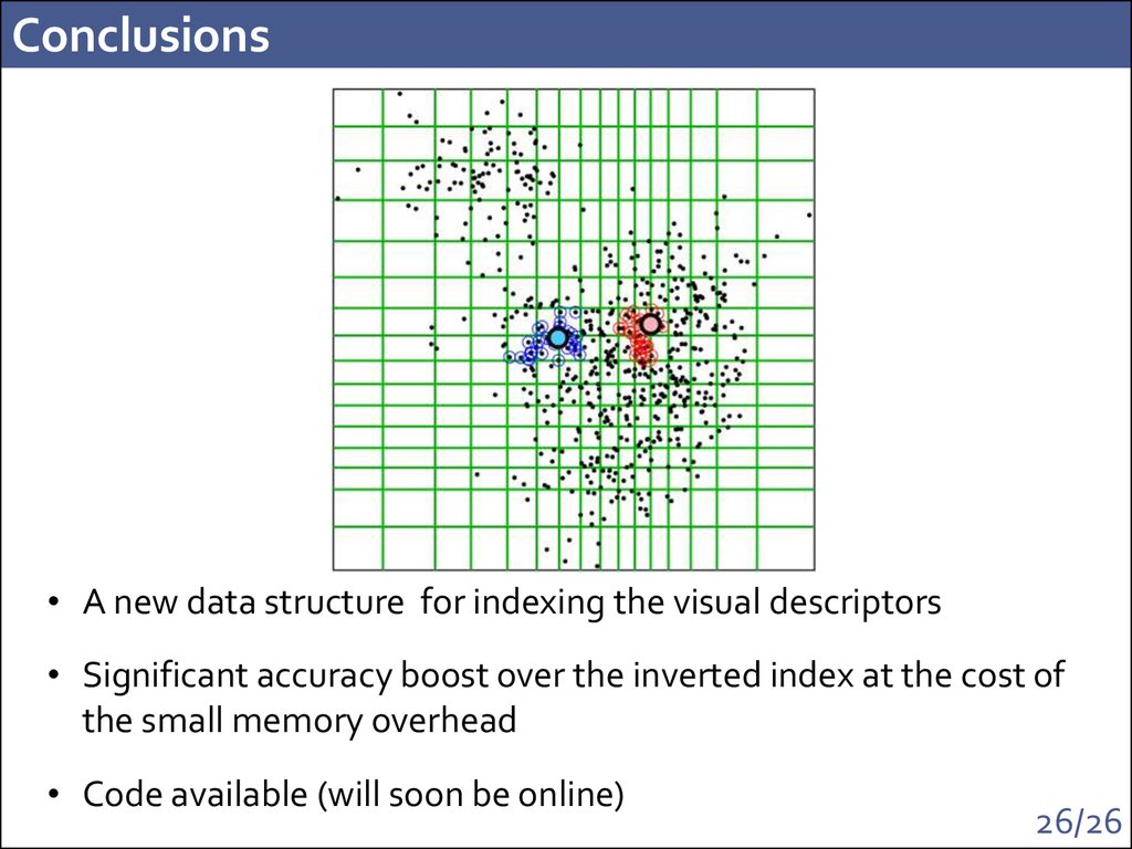
26. Conclusions
• A new data structure for indexing the visual descriptors• Significant accuracy boost over the inverted index at the cost of
the small memory overhead
• Code available (will soon be online)
26/26
27. Other usage scenarios
(Mostly) straightforward extensions possible:• Large-scale NN search' based approaches:
Holistic high dimensional image descriptors: GISTs, VLADs, Fisher
vectors, classemes…
Pose descriptors
Other multimedia
• Additive norms and kernels: L1, Hamming, Mahalanobis, chi-square
kernel, intersection kernel, etc.
27/26










 Программирование

