5.59M

Категория: $Математика$ Математика

Statistics for business and economics. Chapter

1.

CHAPTER 3
STATISTICS FOR BUSINESS AND ECONOMICS 13e Anderson,
David R 2017

2.

Descriptive Statistics
MEASURE OF
LOCATION
MEASURES OF
VARIABILITY
MEASURES OF
DISTRIBUTION
SUMMARIES
AND BOX PLOTS
MEASURES OF
ASSOCIATION

Statistics in Practice
■ Toy and accessory company, that designs and imports products for infants
– Product lines: teddy bears, mobiles, musical toys, rattles and security blankets
– Using high quality color, texture and sound
■ Uses independent representative to sell products. Represented in more than 1000
retail outlets in US
Biggest Challenge, Cash Flow Management

4.

Statistics in Practice
■ Company sets the following goals
– The average age for outstanding invoices should not exceed 45 days
– And the dollar value of invoices more than 60 days old should not exceed 5%
of the dollar value of all accounts receivable
■ Company can use Descriptive Statistics tools to achieve its goals
– Mean
40 days
– Median
35 Days
– Mode
31 days
■ What do these results mean?

5.

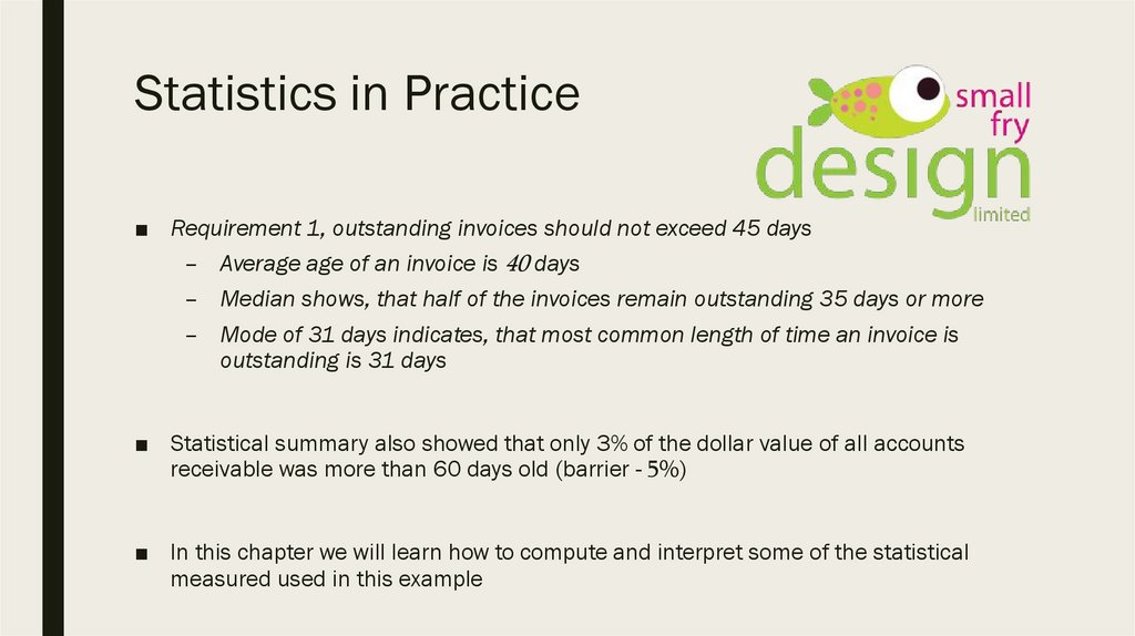
Statistics in Practice
■ Requirement 1, outstanding invoices should not exceed 45 days
– Average age of an invoice is 40 days
– Median shows, that half of the invoices remain outstanding 35 days or more
– Mode of 31 days indicates, that most common length of time an invoice is
outstanding is 31 days
■ Statistical summary also showed that only 3% of the dollar value of all accounts
receivable was more than 60 days old (barrier - 5%)
■ In this chapter we will learn how to compute and interpret some of the statistical
measured used in this example

6.

1. Measure of Location
Mean
■ Average value for a variable

7.

1. Measure of Location
Mean
■ Example

8.

1. Measure of Location
Mean
■ Let’s visualize

9.

1. Measure of Location
Mean
■ Problem – mean is highly effected by extreme values
■ For example, lets replace 54 by 114. new mean is 56. What is the problem?

10.

1. Measure of Location
Mean
■ Let’s do another example
■ Mean is $3940
■ However, do every data points have same “weight”?

11.

1. Measure of Location
Weighted Mean
■ Giving each observation a weight that reflects its relative importance
■ Computed as follows

12.

1. Measure of Location
Weighted Mean
■ Example
■ What is the average price of meat?

13.

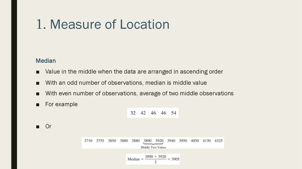
1. Measure of Location
Median
■ Value in the middle when the data are arranged in ascending order
■ With an odd number of observations, median is middle value
■ With even number of observations, average of two middle observations
■ For example
■ Or

14.

1. Measure of Location
Geometric Mean
■ Measure of location that is calculated by finding the nth root of the product of n
values
■ Often used in analyzing growth rates in financial data. Where arithmetic mean or
average value will provide misleading results

15.

1. Measure of Location
Geometric Mean
■ Example
■ If we start with $100
■ End of 1 year our balance is $77.90
■ Beginning of 2 year, starting balance is $77.90. If growth rate is 28.7%. Then ending
balance of year 2 is $100.26
■ Etc

16.

1. Measure of Location
Geometric Mean
■ example
■ At the end of year 10 ending balance can be calculated by using Growth Factor:
■ Therefore growth factor is 1,334493
■ Geometric mean is:

17.

1. Measure of Location
Geometric Mean
■ Example
■ Using geometric mean, at the end of year 10, average growth rate is 2,93%
■ However, if we use arithmetic mean, growth rate is 5.04%. Using this result can be
misleading
■ If average growth rate is 5,04%, at the end of year 10 our initial investment of 100$
would have been $163.51. When we have calculated that it is $133,45

18.

1. Measure of Location
Mode
■ It is the value that occurs with greatest frequency
■ Provide information about how the data is spread over the interval from the smallest
value to the largest
■ Our previous example
■ Mode is $3880

19.

1. Measure of Location
Percentile
■ Provides information about how the data are spread over the interval from the
smallest value to the largest value
■ Pth percentile divides the data into two parts: approximately p% of the observations
are less than the pth percentile, and approximately (100-p)% of the observations are
greater than the pth percentile
■ For example the test results (SAT)
■ Student received 630 points. Is it a bad or good result?
■ We can't say anything if we don’t know other results to compare it to
■ If we know 630 points corresponds to the 82nd percentile, we know that
approximately 82% of the applicants scored lower than this individual, and
approximately 18% of the applicants scored higher than this individual

20.

1. Measure of Location
Percentile
■ Formula
■ If we want to calculate 80th percentile for the data provided below

21.

1. Measure of Location
Percentile
■ 80the percentile would be
■ 10th position value is 4050. plus .4 or 40% of the value to the next one. That is:

22.

1. Measure of Location
Quartiles
■ It is often desired to divide a data in set of four parts, each containing 25% of the
data
■ These division points are referred to as the quartiles
– Q1 = first quartile, or 25th percentile
– Q2 = second quartile, or 50th percentile (also the median)
– Q3 = third quartile, or 75th percentile
■ Example:

23.

2. Measurement of Variability
■ In addition to measures of location, we need to take into account the measures of
variability or dispersion
■ Let’s assume that we have two different suppliers
■ After several months of operation, we find out that mean number of daus required
to fill orders is 10 days for bot of suppliers
■ Which supplier is better?
■ Let’s look at histogram

24.

2. Measurement of Variability
■ What can we say now?

25.

2. Measurement of Variability
■ We need to measure the variability

26.

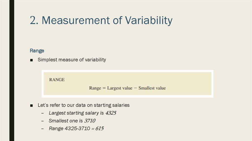
2. Measurement of Variability
Range
■ Simplest measure of variability
■ Let’s refer to our data on starting salaries
– Largest starting salary is 4325
– Smallest one is 3710
– Range 4325-3710 = 615

27.

2. Measurement of Variability
Interquartile Range
■ A measure of variability that overcomes the dependency on extreme values
■ Interquartile range is the range for the middle 50% of the data
■ For our data
– Q3 is 4000
– Q1 is 3865
– IQR is 135

28.

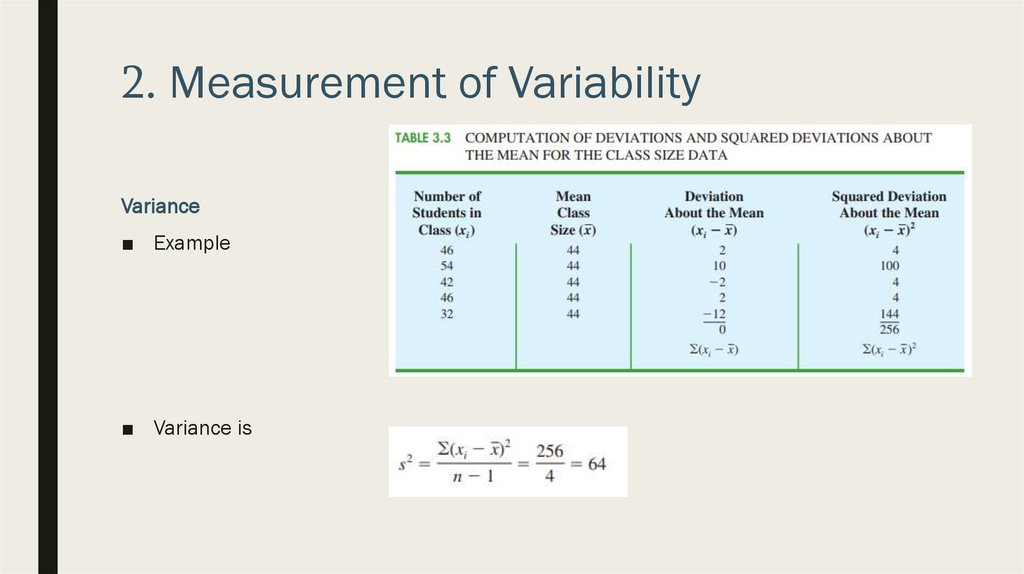
2. Measurement of Variability
Variance
■ A measure of variability that utilizes all the data
■ Measure by the difference between the value of each observation and the mean
■ Population
■ Sample

29.

2. Measurement of Variability
Variance
■ Example
■ Variance is

30.

2. Measurement of Variability
Standard Variance
■ Positive square root of the variance
■ In our case it is:

31.

2. Measurement of Variability
Coefficient of Variation
■ Indicates how large the standard deviation is relative to the mean
■ Formula
■ In our example
– (165,65/3940)*100 = 4,2%
■ Therefore sample standard deviation is 4.2% of the value of the sample mean

32.

3. Measures of Distribution Shape, Relative
Location and Detecting Outliers
■ Aside from the measures of
location and variability for the data,
we also care for a measure of the
shape of a distribution
■ An important numerical measure of
the shape of the distribution is
called skewness

33.

3. Measures of Distribution Shape, Relative
Location and Detecting Outliers
Distribution Shape
■ Formula itself is complicated
■ But histogram helps us to inspect it
visually

34.

3. Measures of Distribution Shape, Relative
Location and Detecting Outliers
Distribution Shape
■ For e symmetric distribution, the mean
and the median are equal
■ When it is skewed positively, the mean
will usually be greater than the median
■ When negative, the mean will usually
be less than the median
■ Panel D, the mean is $77.60 and the
median is $59.70

35.

3. Measures of Distribution Shape, Relative
Location and Detecting Outliers
Z-scores
■ In addition to measures of location, variability and the shape, we are also interested
in the relative location of values within a data set
■ It will help us determine how far a particular value is from the mean
■ Using both mean and standard deviation, we can determine the relative location of
any observation
■ Formula:

36.

3. Measures of Distribution Shape, Relative
Location and Detecting Outliers
Z-scores
■ Example
■ Z-score of 1.2 means, indicates, that xi is 1.2 standard deviations greater than the
sample mean

37.

3. Measures of Distribution Shape, Relative
Location and Detecting Outliers
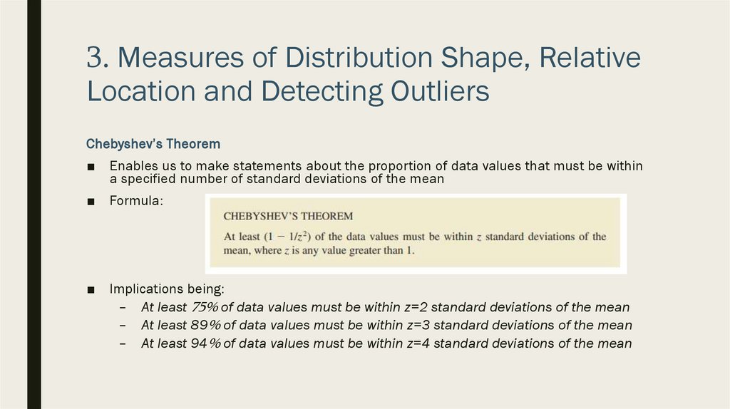
Chebyshev’s Theorem
■ Enables us to make statements about the proportion of data values that must be within
a specified number of standard deviations of the mean
■ Formula:
■ Implications being:
– At least 75% of data values must be within z=2 standard deviations of the mean
– At least 89% of data values must be within z=3 standard deviations of the mean
– At least 94% of data values must be within z=4 standard deviations of the mean

38.

3. Measures of Distribution Shape, Relative
Location and Detecting Outliers
Chebyshev’s Theorem
■ Example
■ Test scores for 100 sudents indicate, that mean is 70 points and standard deviation
of 5
■ What portion of students should be between 60-80 points?
■ Answer:
– 60 is 2 standard deviations from the mean
– Therefore 75%

39.

3. Measures of Distribution Shape, Relative
Location and Detecting Outliers
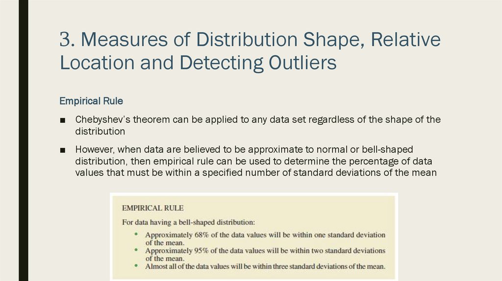
Empirical Rule
■ Chebyshev’s theorem can be applied to any data set regardless of the shape of the
distribution
■ However, when data are believed to be approximate to normal or bell-shaped
distribution, then empirical rule can be used to determine the percentage of data
values that must be within a specified number of standard deviations of the mean

40.

3. დისტრიბუციის გაზომვა
ემპირიული კანონი

41.

3. Measures of Distribution Shape, Relative
Location and Detecting Outliers
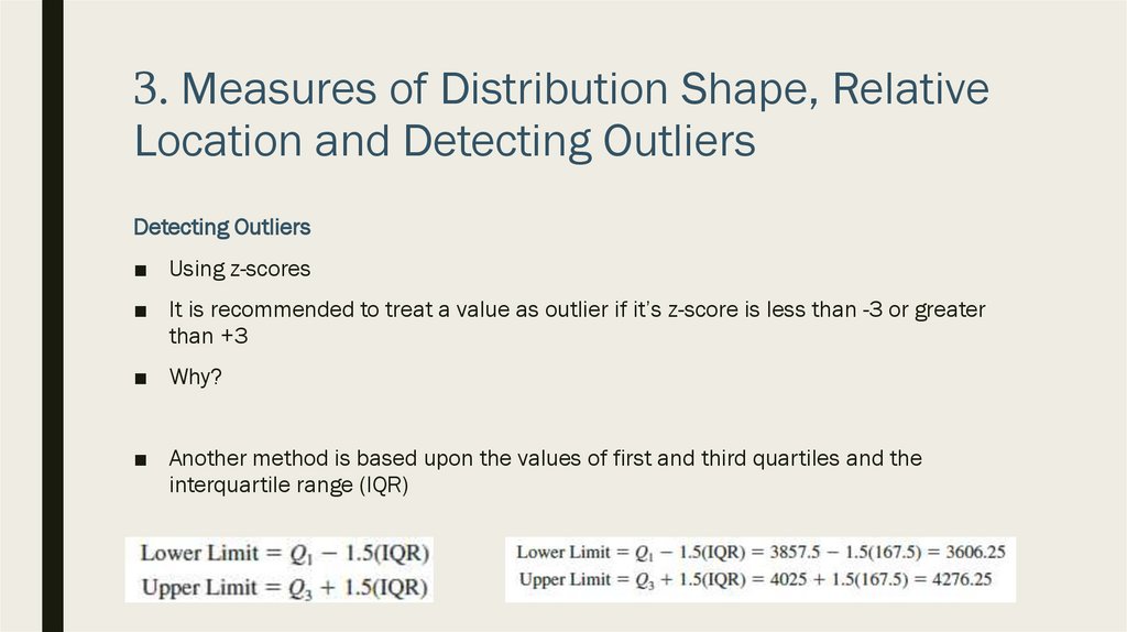
Detecting Outliers
■ Sometimes a data set will have one or more observations with unusually large or
unusually small values
■ We need to identify outliers and review them carefully
■ Outlier may be
– Value that has been incorrectly recorded
– Incorrectly included in the data set
– It may be recoded correctly and may belong to the data set, but may be
unusual data value
■ Standardized values (z-scores) can be used to identify outliers

42.

3. Measures of Distribution Shape, Relative
Location and Detecting Outliers
Detecting Outliers
■ Using z-scores
■ It is recommended to treat a value as outlier if it’s z-score is less than -3 or greater
than +3
■ Why?
■ Another method is based upon the values of first and third quartiles and the
interquartile range (IQR)

43.

4. Five-Number Summaries and Box
Plots
■ Based on summary statistics
■ We will use
– Five-number summary
– And box plots

44.

4. Five-Number Summaries and Box
Plots
Five-Number Summary
■ We need:
– Smallest value
– First quartile (Q1)
– Median (Q2)
– Third quartile (Q3)
– Largest value

45.

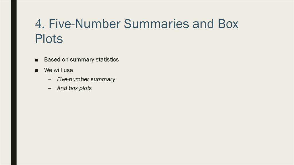
4. Five-Number Summaries and Box
Plots
Five-Number Summary
■ Example
■ We know that: Q1=3857, Q2=3905, Q3=4025
■ Therefore five-number summary results are:
■ Starting salary minimum is 3710 and largest one is 4325 შორის
■ Median, or the middle value is 3905
■ Q1 and Q3 show that approximately 50% of the starting salaries are between 3857,5
and 4025

46.

4. Five-Number Summaries and Box
Plots
Box Plot
■ Graphical representation of five-number summary

47.

4. Five-Number Summaries and Box
Plots
Box Plot
■ Example

48.

5. Measures of Association between
Two Variables
■ Thus far we have examined numerical methods used to summarize the data for one
variable at a time
■ Often we need to make a decision based on the relationship between two variables

49.

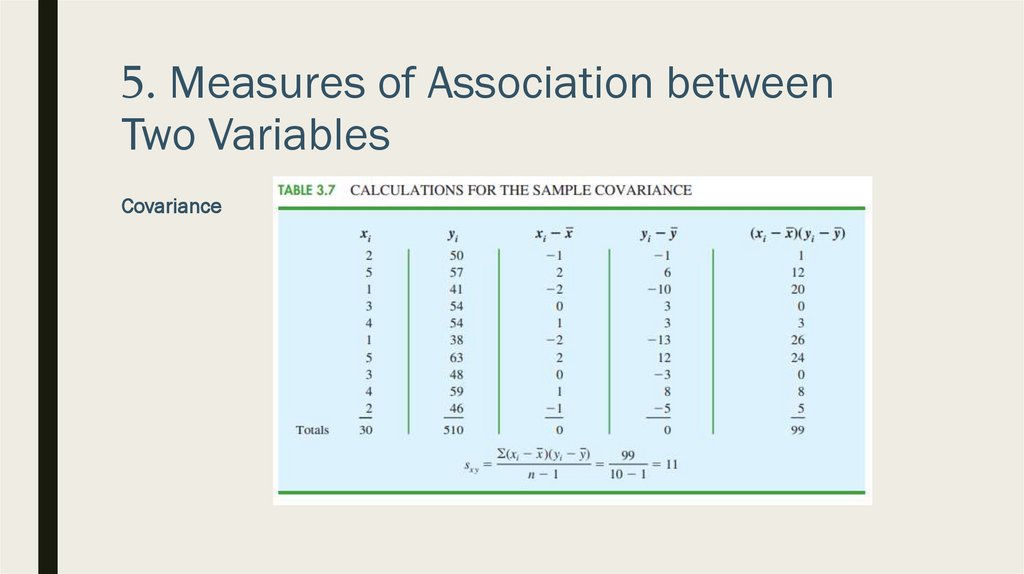
5. Measures of Association between
Two Variables
Covariance
■ Descriptive measure of the linear association between two variables
■ Let’s look at the relationship between TV commercials and sales at the store the
following week

50.

5. Measures of Association between
Two Variables
Covariance

51.

5. Measures of Association between
Two Variables
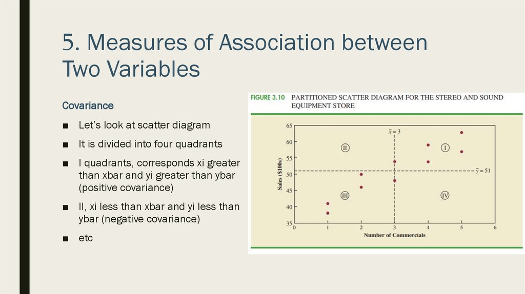
Covariance
■ Let’s look at scatter diagram
■ It is divided into four quadrants
■ I quadrants, corresponds xi greater
than xbar and yi greater than ybar
(positive covariance)
■ II, xi less than xbar and yi less than
ybar (negative covariance)
■ etc

52.

5. Measures of Association between
Two Variables
Covariance

53.

5. Measures of Association between
Two Variables
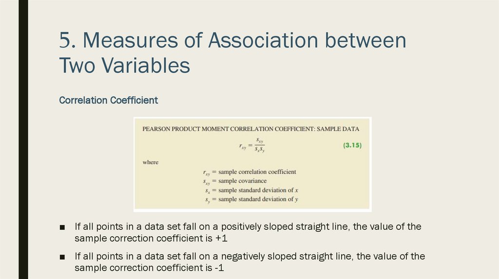
Correlation Coefficient
■ If all points in a data set fall on a positively sloped straight line, the value of the
sample correction coefficient is +1
■ If all points in a data set fall on a negatively sloped straight line, the value of the
sample correction coefficient is -1