844.94K

Категория:

Программирование

Основы Python. Пакет NumPy

2.

PIP: PIP Installs Packages
• sudo pip install packagename
sudo pip uninstall packagename
• cd C:\Python27\Scripts\
pip install packagename
pip uninstall packagename
• pip install numpy
Linux
Windows

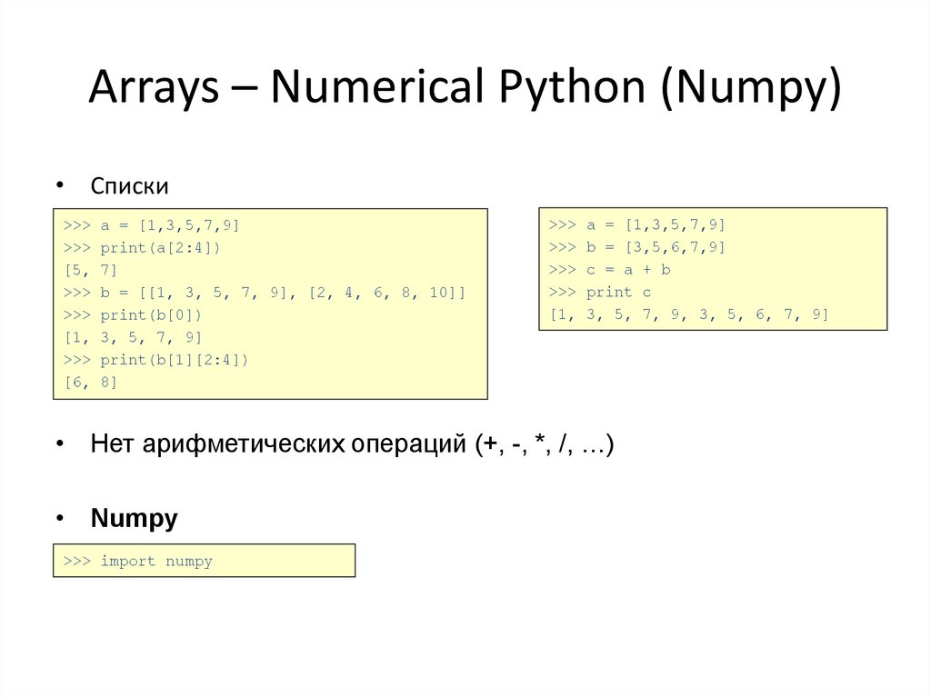
Arrays – Numerical Python (Numpy)
• Списки
>>>
>>>
[5,
>>>
>>>
[1,
>>>
[6,
a = [1,3,5,7,9]
print(a[2:4])
7]
b = [[1, 3, 5, 7, 9], [2, 4, 6, 8, 10]]
print(b[0])
3, 5, 7, 9]
print(b[1][2:4])
8]
>>>
>>>
>>>
>>>
[1,
a = [1,3,5,7,9]
b = [3,5,6,7,9]
c = a + b
print c
3, 5, 7, 9, 3, 5, 6, 7, 9]
• Нет арифметических операций (+, -, *, /, …)
• Numpy
>>> import numpy

4.

Numpy – N-dimensional Array manipulations
NumPy – основная библиотека для научных расчетов в Python:
• поддержка многомерных массивов (арифметика, подмассивы, преобразования)
включает 3 доп. библиотеки с процедурами для:
• линейной алгебры (решение СЛАУ)
• дискретное преобразование Фурье
• работа со случайными числами

5.

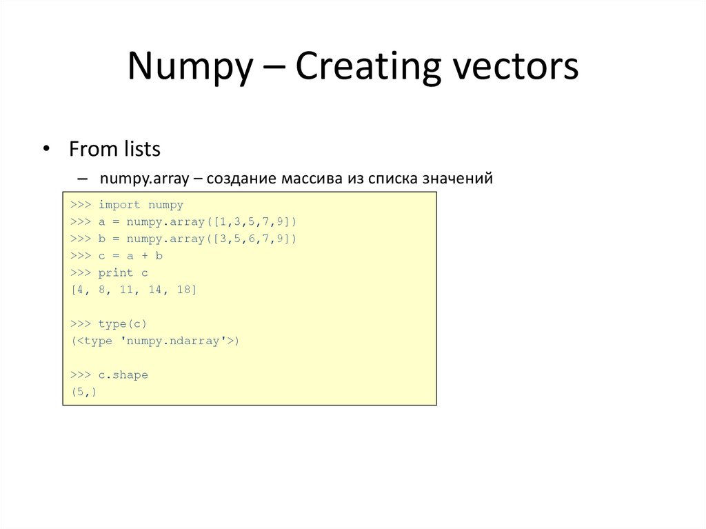
Numpy – Creating vectors
• From lists
– numpy.array – создание массива из списка значений
>>>
>>>
>>>
>>>
>>>
[4,
import numpy
a = numpy.array([1,3,5,7,9])
b = numpy.array([3,5,6,7,9])
c = a + b
print c
8, 11, 14, 18]
>>> type(c)
(<type 'numpy.ndarray'>)
>>> c.shape
(5,)

6.

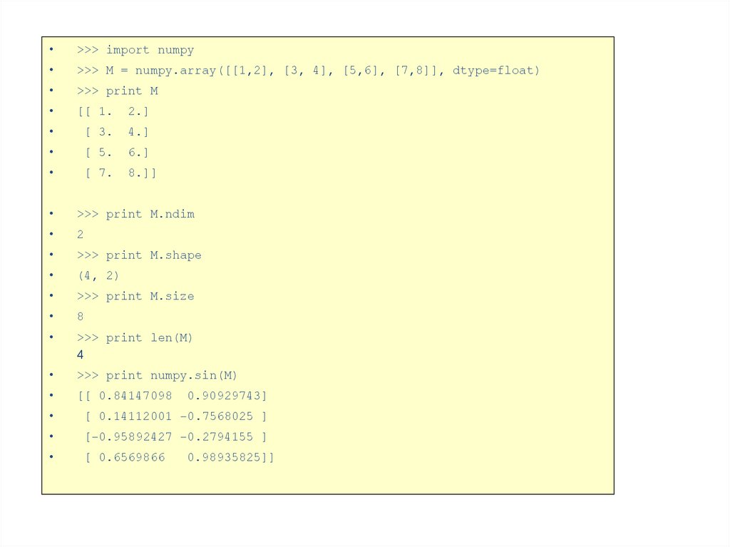
>>> import numpy
>>> M = numpy.array([[1,2], [3, 4], [5,6], [7,8]], dtype=float)
>>> print M
[[ 1.
2.]
[ 3.
4.]
[ 5.
6.]
[ 7.
8.]]
>>> print M.ndim
2
>>> print M.shape
(4, 2)
>>> print M.size
8
>>> print len(M)
4
>>> print numpy.sin(M)
[[ 0.84147098
0.90929743]
[ 0.14112001 -0.7568025 ]
[-0.95892427 -0.2794155 ]
[ 0.6569866
0.98935825]]

7.

Numpy – Creating matrices
>>> L = [[1, 2, 3], [3, 6, 9], [2, 4, 6]] # create a list
>>> a = numpy.array(L) # convert a list to an array
>>> print a
[[1 2 3]
# or directly as matrix
[3 6 9]
>>> M = numpy.array([[1, 2], [3, 4]])
[2 4 6]]
>>> print M.shape
>>> print a.shape
(2,2)
(3, 3)
>>> print M.dtype
>>> print a.dtype # get type of an array
dtype('int64')
dtype('int64')
#only one type
>>> M[0,0] = "hello"
Traceback (most recent call last):
File "<stdin>", line 1, in <module>
ValueError: invalid literal for long() with base 10:
>>> M = numpy.array([[1, 2], [3, 4]], dtype=complex)
>>> print M
array([[ 1.+0.j, 2.+0.j],
[ 3.+0.j, 4.+0.j]])

8.

Numpy – Matrices use
>>> print(a)
[[1 2 3]
[3 6 9]
[2 4 6]]
>>> print(a[0]) # this is just like a list of lists
[1 2 3]
>>> print(a[1, 2]) # arrays can be given comma separated indices
9
>>> print(a[1, 1:3]) # and slices
[6 9]
>>> print(a[:,1])
[2 6 4]
>>> a[1, 2] = 7
>>> print(a)
[[1 2 3]
[3 6 7]
[2 4 6]]
>>> a[:, 0] = [0, 9, 8]
>>> print(a)
[[0 2 3]
[9 6 7]
[8 4 6]]

9.

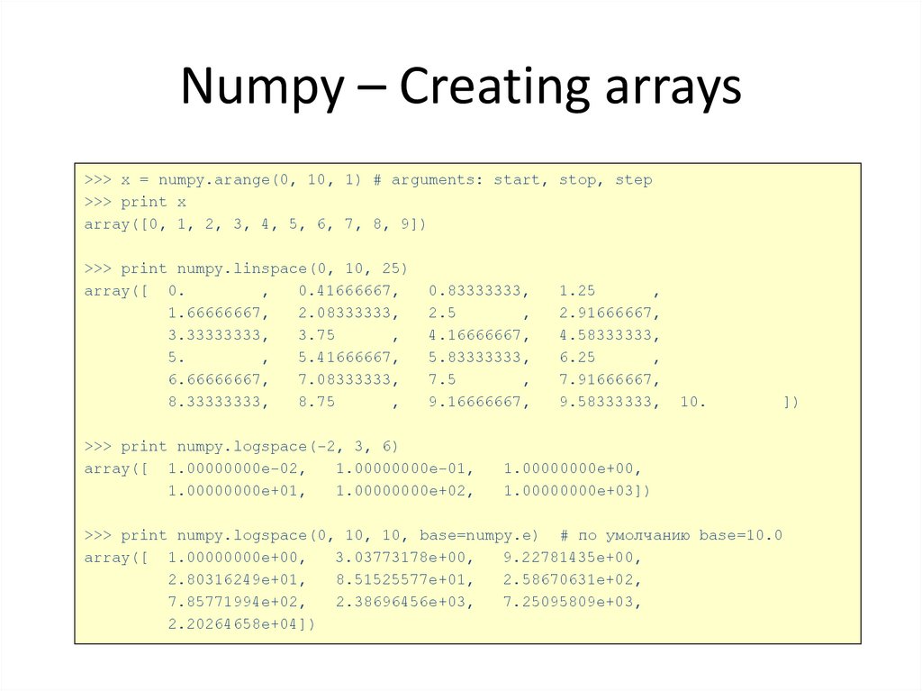
Numpy – Creating arrays
>>> x = numpy.arange(0, 10, 1) # arguments: start, stop, step
>>> print x
array([0, 1, 2, 3, 4, 5, 6, 7, 8, 9])
>>> print numpy.linspace(0, 10, 25)
array([ 0.
,
0.41666667,
1.66666667,
2.08333333,
3.33333333,
3.75
,
5.
,
5.41666667,
6.66666667,
7.08333333,
8.33333333,
8.75
,
0.83333333,
2.5
,
4.16666667,
5.83333333,
7.5
,
9.16666667,
>>> print numpy.logspace(-2, 3, 6)
array([ 1.00000000e-02,
1.00000000e-01,
1.00000000e+01,
1.00000000e+02,
1.25
,
2.91666667,
4.58333333,
6.25
,
7.91666667,
9.58333333,
10.
])
1.00000000e+00,
1.00000000e+03])
>>> print numpy.logspace(0, 10, 10, base=numpy.e) # по умолчанию base=10.0
array([ 1.00000000e+00,
3.03773178e+00,
9.22781435e+00,
2.80316249e+01,
8.51525577e+01,
2.58670631e+02,
7.85771994e+02,
2.38696456e+03,
7.25095809e+03,
2.20264658e+04])

10.

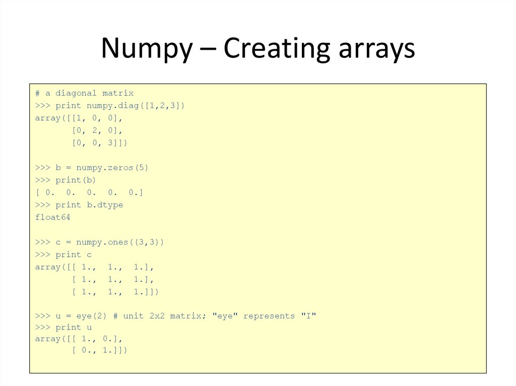
Numpy – Creating arrays
# a diagonal matrix
>>> print numpy.diag([1,2,3])
array([[1, 0, 0],
[0, 2, 0],
[0, 0, 3]])
>>> b = numpy.zeros(5)
>>> print(b)
[ 0. 0. 0. 0. 0.]
>>> print b.dtype
float64
>>> c = numpy.ones((3,3))
>>> print c
array([[ 1., 1., 1.],
[ 1., 1., 1.],
[ 1., 1., 1.]])
>>> u = eye(2) # unit 2x2 matrix; "eye" represents "I"
>>> print u
array([[ 1., 0.],
[ 0., 1.]])

11.

Numpy – array creation and use
>>> d = numpy.arange(5)
>>> print(d)
[0 1 2 3 4]
# just like range()
>>> d[1] = 9.7
>>> print(d) # arrays keep their type even if elements changed
[0 9 2 3 4]
>>> print(d*0.4) # operations create a new array, with new type
[ 0.
3.6 0.8 1.2 1.6]
>>> d = numpy.arange(5, dtype=float)
>>> print(d)
[ 0. 1. 2. 3. 4.]

12.

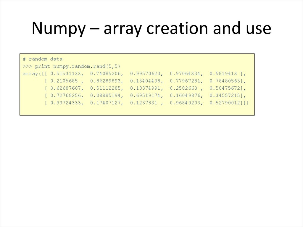
Numpy – array creation and use
# random data
>>> print numpy.random.rand(5,5)
array([[ 0.51531133, 0.74085206,
[ 0.2105685 , 0.86289893,
[ 0.62687607, 0.51112285,
[ 0.72768256, 0.08885194,
[ 0.93724333, 0.17407127,
0.99570623,
0.13404438,
0.18374991,
0.69519174,
0.1237831 ,
0.97064334,
0.77967281,
0.2582663 ,
0.16049876,
0.96840203,
0.5819413 ],
0.78480563],
0.58475672],
0.34557215],
0.52790012]])

13.

Numpy – Creating arrays
• Чтение из файла
sample.txt:
"Stn", "Datum", "Tg", "qTg", "Tn", "qTn", "Tx", "qTx"
001, 19010101,
-49, 00,
-68, 00,
-22, 40
001, 19010102,
-21, 00,
-36, 30,
-13, 30
001, 19010103,
-28, 00,
-79, 30,
-5, 20
001, 19010104,
-64, 00,
-91, 20,
-10, 00
001, 19010105,
-59, 00,
-84, 30,
-18, 00
001, 19010106,
-99, 00, -115, 30,
-78, 30
001, 19010107,
-91, 00, -122, 00,
-66, 00
001, 19010108,
-49, 00,
-94, 00,
-6, 00
001, 19010109,
11, 00,
-27, 40,
42, 00
...
>>> data = numpy.genfromtxt('sample.txt', delimiter=',', skip_header=1)
>>> print data.shape
(25568, 8)

14.

Numpy – Creating arrays
• Сохранение в файл
>>> numpy.savetxt('datasaved.txt', data)
datasaved.txt:
1.000000000000000000e+00 1.901010100000000000e+07 -4.900000000000000000e+01
0.000000000000000000e+00 -6.800000000000000000e+01 0.000000000000000000e+00
-2.200000000000000000e+01 4.000000000000000000e+01
1.000000000000000000e+00 1.901010200000000000e+07 -2.100000000000000000e+01
0.000000000000000000e+00 -3.600000000000000000e+01 3.000000000000000000e+01
-1.300000000000000000e+01 3.000000000000000000e+01
1.000000000000000000e+00 1.901010300000000000e+07 -2.800000000000000000e+01
0.000000000000000000e+00 -7.900000000000000000e+01 3.000000000000000000e+01
-5.000000000000000000e+00 2.000000000000000000e+01

15.

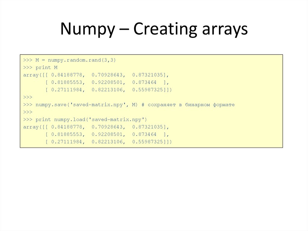
Numpy – Creating arrays
>>> M = numpy.random.rand(3,3)
>>> print M
array([[ 0.84188778, 0.70928643, 0.87321035],
[ 0.81885553, 0.92208501, 0.873464 ],
[ 0.27111984, 0.82213106, 0.55987325]])
>>>
>>> numpy.save('saved-matrix.npy', M) # сохраняет в бинарном формате
>>>
>>> print numpy.load('saved-matrix.npy')
array([[ 0.84188778, 0.70928643, 0.87321035],
[ 0.81885553, 0.92208501, 0.873464 ],
[ 0.27111984, 0.82213106, 0.55987325]])

16.

Numpy – array methods
>>> print arr.sum()
145
>>> print arr.mean()
14.5
>>> print arr.std()
2.8722813232690143
>>> print arr.max()
19
>>> print arr.min()
10

17.

Numpy – array methods - sorting
>>> arr = numpy.array([4.5, 2.3, 6.7, 1.2, 1.8, 5.5])
>>> arr.sort() # acts on array itself
>>> print(arr)
[ 1.2 1.8 2.3 4.5 5.5 6.7]
>>> x = numpy.array([4.5, 2.3, 6.7, 1.2, 1.8, 5.5])
>>> y = numpy.sort(x)
>>> print(y)
[ 1.2 1.8 2.3 4.5 5.5 6.7]
>>> print(x)
[ 4.5 2.3 6.7 1.2 1.8 5.5]

18.

Numpy – array functions
>>> print arr.sum()
45
>>> print numpy.sum(arr)
45
>>> x = numpy.array([[1,2],[3,4]])
>>> print x
[[1 2]
[3 4]]
>>> print numpy.log10(x)
[[ 0.
0.30103
]
[ 0.47712125 0.60205999]]

19.

Numpy – array operations
>>> a = numpy.array([[1.0, 2.0], [4.0, 3.0]])
>>> print a
[[ 1. 2.]
[ 3. 4.]]
>>> print a.transpose()
array([[ 1., 3.],
[ 2., 4.]])
>>> print numpy.inv(a)
array([[-2. , 1. ],
[ 1.5, -0.5]])
>>> j = numpy.array([[0.0, -1.0], [1.0, 0.0]])
>>> print j
array([[0., -1.],
[1., 0.]])
>>> print j*j # element product
array([[0., 1.],
[1., 0.]])
>>> print numpy.dot(j, j) # matrix product
array([[-1., 0.],
[ 0., -1.]])

20.

Numpy – arrays, matrices
В NumPy есть специальный тип matrix для работы с матрицами. Матрицы могут
быть созданы вызовом matrix() или mat() или преобразованы из двумерных
массивов методом asmatrix().
>>> import numpy
>>> m = numpy.mat([[1,2],[3,4]])
>>> a = numpy.array([[1,2],[3,4]])
>>> m = numpy.mat(a)
>>> a = numpy.array([[1,2],[3,4]])
>>> m = numpy.asmatrix(a)

21.

Numpy – matrices
>>> a = numpy.array([[1,2],[3,4]])
>>> m = numpy.mat(a) # convert 2-d array to matrix
>>> print a[0]
array([1, 2])
>>> print m[0]
matrix([[1, 2]])
# result is 1-dimensional
>>> print a*a
array([[ 1, 4], [ 9, 16]])
>>> print m*m
matrix([[ 7, 10], [15, 22]])
# element-by-element multiplication
# result is 2-dimensional
# (algebraic) matrix multiplication
>>> print a**3
# element-wise power
array([[ 1, 8], [27, 64]])
>>> print m**3
# matrix multiplication m*m*m
matrix([[ 37, 54], [ 81, 118]])
>>> print m.T
# transpose of the matrix
matrix([[1, 3], [2, 4]])
>>> print m.H
# conjugate transpose (differs from .T for complex matrices)
matrix([[1, 3], [2, 4]])
>>> print m.I
# inverse matrix
matrix([[-2. , 1. ], [ 1.5, -0.5]])

22.

Numpy – Fourier
>>> a = linspase(0,1,11)
>>> print a
[ 0.
0.1 0.2 0.3 0.4
>>> from numpy.fft
>>> b = fft(a)
>>> print b
[ 5.50+0.j
-0.55+0.25117658j
-0.55-0.47657771j
0.5
0.6
0.7
0.8
0.9
1. ]
import fft, ifft
-0.55+1.87312798j -0.55+0.85581671j -0.55+0.47657771j
-0.55+0.07907806j -0.55-0.07907806j -0.55-0.25117658j
-0.55-0.85581671j -0.55-1.87312798j]
>>> print(ifft(b))
[ 1.61486985e-15+0.j
3.00000000e-01+0.j
6.00000000e-01+0.j
9.00000000e-01+0.j
1.00000000e-01+0.j
4.00000000e-01+0.j
7.00000000e-01+0.j
1.00000000e+00+0.j]
2.00000000e-01+0.j
5.00000000e-01+0.j
8.00000000e-01+0.j

23.

Plotting - matplotlib
>>> import matplotlib.pyplot as plt

24.

Matplotlib.pyplot basic example
import matplotlib.pyplot as plt
plt.plot([1,3,2,4])
plt.ylabel('some numbers')
plt.show()

25.

Matplotlib.pyplot basic example
import numpy
import matplotlib.pyplot as plt
x = numpy.linspace(0, 5, 10)
y = x ** 2
plt.plot(x, y, 'r')
plt.xlabel('x')
plt.ylabel('y')
plt.title('title')
plt.show()

26.

27.

Matplotlib.pyplot basic example
x = numpy.linspace(0, 5, 10)
y = x ** 2
plt.subplot(1,2,1)
plt.plot(x, y, ’r--’)
plt.subplot(1,2,2)
plt.plot(y, x, ’g*-’)
plt.show()

28.

x = numpy.linspace(0, 5, 2)
plt.plot(x, x+1, color="red", alpha=0.5) # half-transparant red
plt.plot(x, x+2, color="#1155dd") # RGB hex code for a bluish color
plt.plot(x, x+3, color="#15cc55") # RGB hex code for a greenish color
plt.show()

29.

plt.plot(x,
plt.plot(x,
plt.plot(x,
plt.plot(x,
x+1,
x+2,
x+3,
x+4,
color="blue",
color="blue",
color="blue",
color="blue",
linewidth=0.25)
linewidth=0.50)
linewidth=1.00)
linewidth=2.00)
# possible linestype options ‘-‘, ‘{’, ‘-.’, ‘:’, ‘steps’
plt.plot(x, x+5, color="red", lw=2, linestyle=’-’)
plt.plot(x, x+6, color="red", lw=2, ls=’-.’)
plt.plot(x, x+7, color="red", lw=2, ls=’:’)
# possible marker
plt.plot(x, x+ 9,
plt.plot(x, x+10,
plt.plot(x, x+11,
plt.plot(x, x+12,
symbols: marker = ’+’, ’o’, ’*’, ’s’, ’,’, ’.’, ’1’, ’2’, ’3’, ’4’, ...
color="green", lw=2, ls=’*’, marker=’+’)
color="green", lw=2, ls=’*’, marker=’o’)
color="green", lw=2, ls=’*’, marker=’s’)
color="green", lw=2, ls=’*’, marker=’1’)
# marker size and color
plt.plot(x, x+13, color="purple", lw=1, ls=’-’, marker=’o’, markersize=2)
plt.plot(x, x+14, color="purple", lw=1, ls=’-’, marker=’o’, markersize=4)
plt.plot(x, x+15, color="purple", lw=1, ls=’-’, marker=’o’, markersize=8, markerfacecolor="red")
plt.plot(x, x+16, color="purple", lw=1, ls=’-’, marker=’s’, markersize=8,
markerfacecolor="yellow", markeredgewidth=2, markeredgecolor="blue")

30.

Matplotlib.pyplot example
import numpy as np
import matplotlib.pyplot as plt
def f(t):
return np.exp(-t) * np.cos(2*np.pi*t)
t1 = np.arange(0.0, 5.0, 0.1)
t2 = np.arange(0.0, 5.0, 0.02)
plt.subplot(211)
plt.plot(t1, f(t1), 'bo', t2, f(t2), 'k')
plt.subplot(212)
plt.plot(t2, np.cos(2*np.pi*t2), 'r--')
plt.show()

31.

Matplotlib.pyplot basic example
fig = plt.figure()
axes1 = fig.add_axes([0.1, 0.1, 0.8, 0.8]) # main axes
axes2 = fig.add_axes([0.2, 0.5, 0.4, 0.3]) # inset axes
x = numpy.linspace(0, 5, 10)
y = x ** 2
# main figure
axes1.plot(x, y, ’r’)
axes1.set_xlabel(’x’)
axes1.set_ylabel(’y’)
axes1.set_title(’title’)
# insert
axes2.plot(y, x, ’g’)
axes2.set_xlabel(’y’)
axes2.set_ylabel(’x’)
axes2.set_title(’insert title’);

32.

Matplotlib.pyplot basic example
Labels and legends and titles
import numpy as np
import matplotlib.pyplot as plt
x = np.arange(0.0, 5.0, 0.1)
plt.plot(x, x**2, 'bo', label='y = x**2')
plt.plot(x, np.cos(2*np.pi*x), 'r--',
label='y = cos(2 pi x)')
plt.legend(loc=0)
plt.xlabel('x')
plt.ylabel('y')
plt.title('title')
plt.show()
plt.legend(loc=0)
plt.legend(loc=1)
plt.legend(loc=2)
plt.legend(loc=3)
plt.legend(loc=4)
#
#
#
#
#
let matplotlib decide
upper right corner
upper left corner
lower left corner
lower right corner

33.

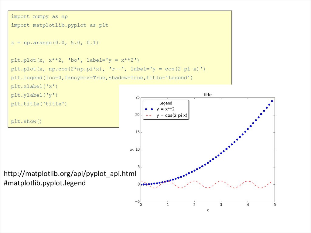
import numpy as np
import matplotlib.pyplot as plt
x = np.arange(0.0, 5.0, 0.1)
plt.plot(x, x**2, 'bo', label='y = x**2')
plt.plot(x, np.cos(2*np.pi*x), 'r--', label='y = cos(2 pi x)')
plt.legend(loc=0,fancybox=True,shadow=True,title='Legend')
plt.xlabel('x')
plt.ylabel('y')
plt.title('title')
plt.show()
http://matplotlib.org/api/pyplot_api.html
#matplotlib.pyplot.legend

34.

Matplotlib.pyplot basic example
plt.plot(x, x**2, 'bo', label='$y = x^2$')
plt.plot(x, np.cos(2*np.pi*x), 'r--', label='$y = \\cos(2 \\pi x)$')
#plt.plot(x, np.cos(2*np.pi*x), 'r--', label=r'$y = \cos(2 \pi x)$')

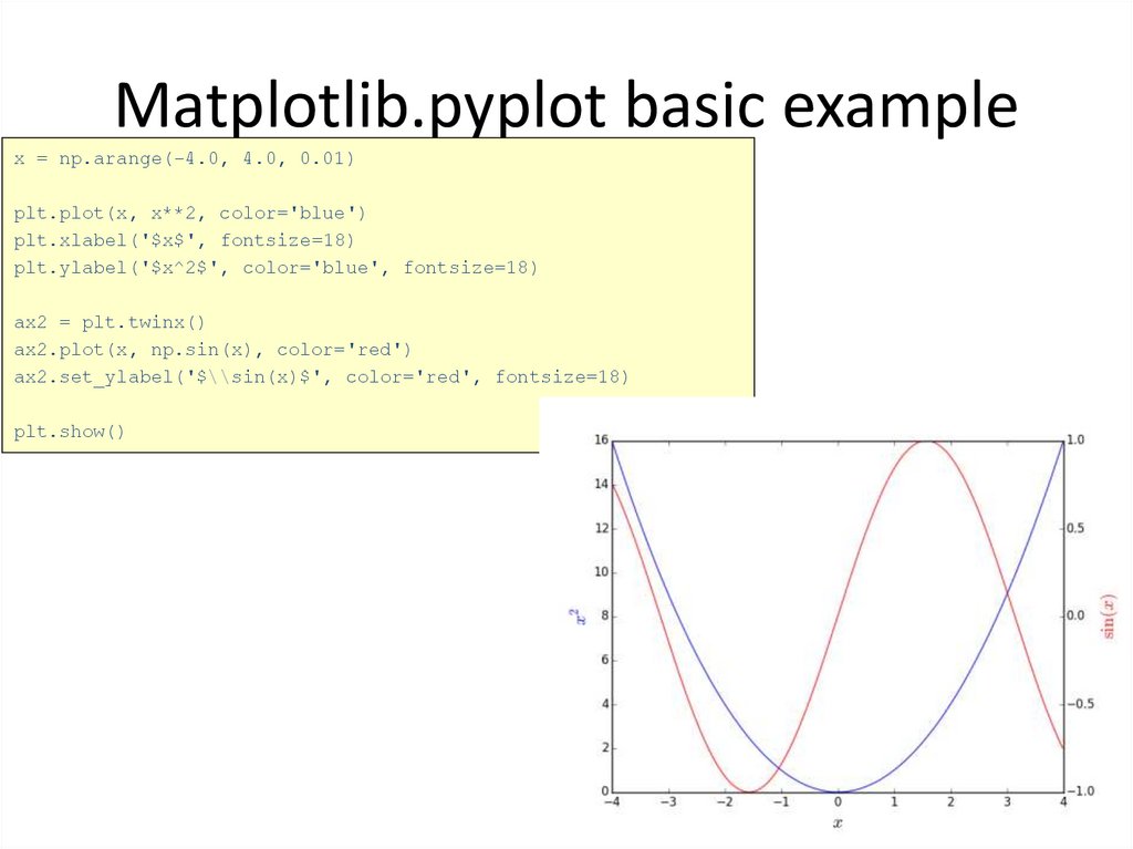
35.

Matplotlib.pyplot basic example
x = np.arange(-4.0, 4.0, 0.01)
plt.plot(x, x**2, color='blue')
plt.xlabel('$x$', fontsize=18)
plt.ylabel('$x^2$', color='blue', fontsize=18)
ax2 = plt.twinx()
ax2.plot(x, np.sin(x), color='red')
ax2.set_ylabel('$\\sin(x)$', color='red', fontsize=18)
plt.show()

36.

Overwhelming annotation
x = np.arange(-2.0, 2.0, 0.01)
plt.plot(x, np.cos(2*np.pi*x))
plt.xlim(-2.1, 2.1)
plt.ylim(-1.5, 1.5)
plt.annotate('-',
plt.annotate('->',
plt.annotate('-|>',
plt.annotate('<->',
plt.annotate('-[',
xy=(-2,1),
xy=(-1,1),
xy=(0,1),
xy=(1,1),
xy=(2,1),
plt.annotate('fancy',
plt.annotate('simple',
plt.annotate('wedge',
plt.annotate('|-|',
plt.show()
xytext=(-1.8,1.3),
xytext=(-0.8,1.3),
xytext=(0,1.3),
xytext=(0.8,1.3),
xytext=(1.8,1.3),
xy=(-1.5,-1),
xy=(-0.5,-1),
xy=(0.5,-1),
xy=(1.5,-1),
arrowprops=dict(arrowstyle='-'))
arrowprops=dict(arrowstyle='->'))
arrowprops=dict(arrowstyle='-|>'))
arrowprops=dict(arrowstyle='<->'))
arrowprops=dict(arrowstyle='-['))
xytext=(-1.5,-1.3),
xytext=(-0.5,-1.3),
xytext=(0.5,-1.3),
xytext=(1.5,-1.3),
arrowprops=dict(arrowstyle='fancy'))
arrowprops=dict(arrowstyle='simple'))
arrowprops=dict(arrowstyle='wedge'))
arrowprops=dict(arrowstyle='|-|'))

37.

Matplotlib.pyplot basic example
x = np.linspace(-1.0, 2.0, 16)
plt.subplot(221)
plt.scatter(x, np.sin(50 * x + 12))
plt.subplot(222)
plt.step(x, x**2)
plt.subplot(223)
plt.bar(x, x**2, width=0.1)
plt.subplot(224)
plt.fill_between(x, x**2, x**3, color='green')
plt.show()