


 Программное обеспечение
Похожие презентации:

")
")
")


Bit strings will be used to identify parts of this tutorial on the computer output
1.
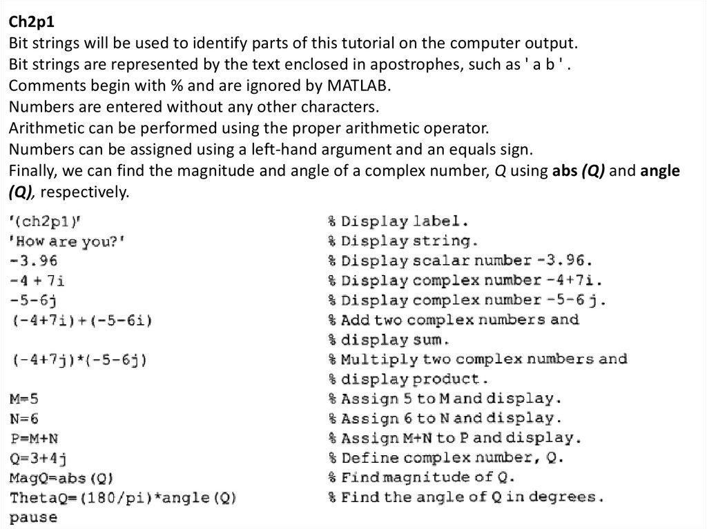
Ch2p1Bit strings will be used to identify parts of this tutorial on the computer output.
Bit strings are represented by the text enclosed in apostrophes, such as ' a b ' .
Comments begin with % and are ignored by MATLAB.
Numbers are entered without any other characters.
Arithmetic can be performed using the proper arithmetic operator.
Numbers can be assigned using a left-hand argument and an equals sign.
Finally, we can find the magnitude and angle of a complex number, Q using abs (Q) and angle
(Q), respectively.
2.
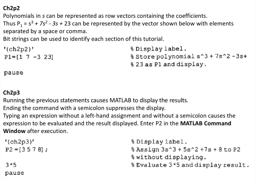
Ch2p2Polynomials in s can be represented as row vectors containing the coefficients.
Thus P1 = s3 + 7s2 - 3s + 23 can be represented by the vector shown below with elements
separated by a space or comma.
Bit strings can be used to identify each section of this tutorial.
Ch2p3
Running the previous statements causes MATLAB to display the results.
Ending the command with a semicolon suppresses the display.
Typing an expression without a left-hand assignment and without a semicolon causes the
expression to be evaluated and the result displayed. Enter P2 in the MATLAB Command
Window after execution.
3.
Ch2p4: factored form to polynomial formAn F(s) in factored form can be represented in polynomial form.
Thus P3 = (s + 2) (s + 5) (s + 6) can be transformed into a polynomial using po1y (V), where
V is a row vector containing the roots of the polynomial and
poly (V) forms the coefficients of the polynomial.
Ch2p5: polynomial form to factored form
We can find roots of polynomials using the roots (V) command.
The roots are returned as a column vector. For example,
find the roots of
5s4 + 7s3 + 9s2-3s + 2 = 0.
4.
Ch2p6: Multiplication of PolynomialsPolynomials can be multiplied together using the conv(a,b) command (standing for convolve).
Thus, P5 = (s3 + 7s2 + 10s + 9)(s4 - 3s3 + 6s2 + 2s + 1) is generated as follows:
Ch2p7: The partial-fraction expansion
The partial-fraction expansion for F(s) = b(s)/a(s) can be found using the
[r, p, k] = residue (b, a) command (r = residue; p = roots of denominator; k = direct quotient,
which is found by dividing polynomials prior to performing a partial fraction expansion).
We expand F(s) = (7s2 + 9s + 12)/[s{s + 7)(s2 + 10s + 100)] as an example.
Using the results from MATLAB yields: F(s) = [(0.2554 - 0.3382i) / (s + 5.0000 - 8.6603i)] +
[(0.2554 + 0.3382i) / (s + 5.0000 + 8.6603i)] – [0.5280/ (s + 7)] + [0.0171/s].
Note
Note : use r instead K
5.
Ch2p9: Creating Transfer FunctionsVector Method, Polynomial Form
A transfer function can be expressed as a numerator polynomial divided by a denominator
polynomial, that is, F(s) = N(s)/D(s). The numerator, N(s), is represented by a row vector,
numf, that contains the coefficients of N(s). Similarly, the denominator, D(s), is represented
by a row vector, denf, that contains the coefficients of D(s).
We form F(s) with the command, F=tf (numf, denf).
We demonstrate with
F(s) = 150(s2 + 2s + 7)/[s{s2 + 5s + 4)].
Notice after executing the tf command, MATLAB prints the transfer function.
6.
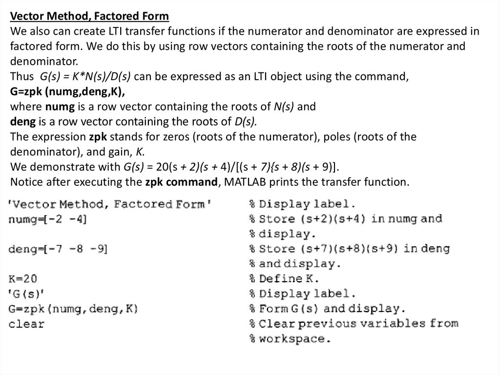
Vector Method, Factored FormWe also can create LTI transfer functions if the numerator and denominator are expressed in
factored form. We do this by using row vectors containing the roots of the numerator and
denominator.
Thus G(s) = K*N(s)/D(s) can be expressed as an LTI object using the command,
G=zpk (numg,deng,K),
where numg is a row vector containing the roots of N(s) and
deng is a row vector containing the roots of D(s).
The expression zpk stands for zeros (roots of the numerator), poles (roots of the
denominator), and gain, K.
We demonstrate with G(s) = 20(s + 2)(s + 4)/[(s + 7){s + 8)(s + 9)].
Notice after executing the zpk command, MATLAB prints the transfer function.
7.
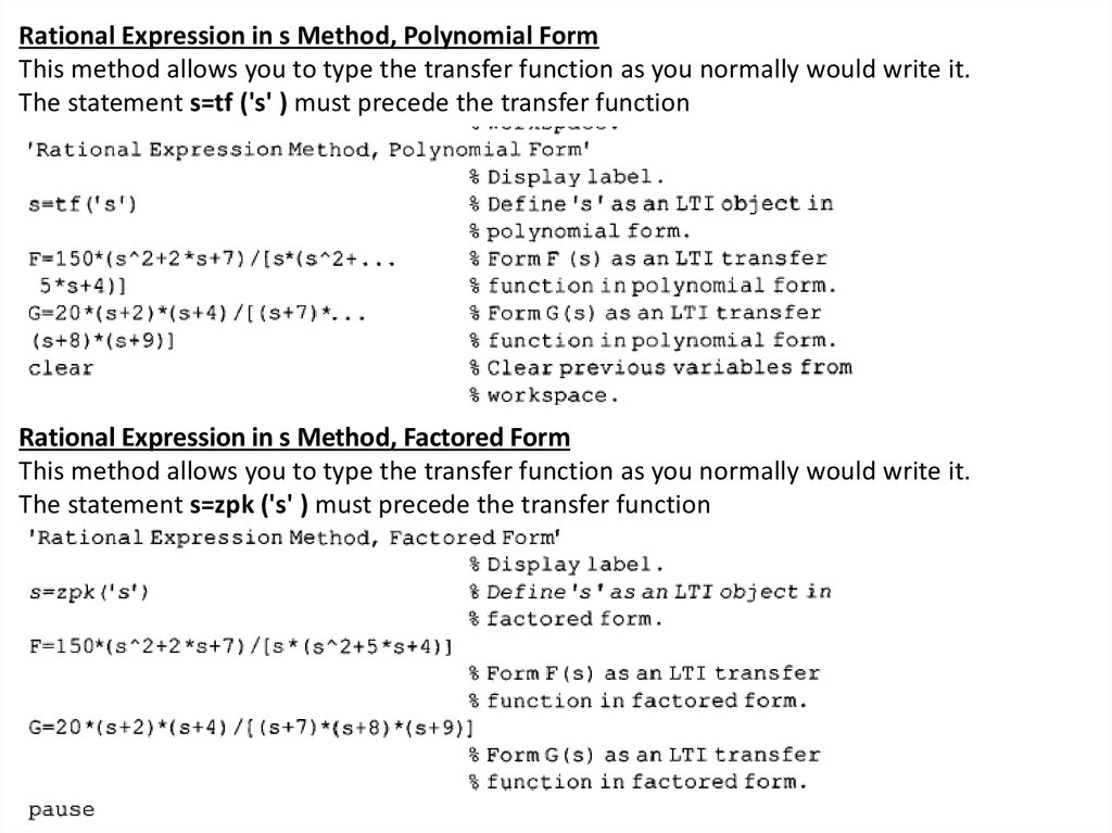
Rational Expression in s Method, Polynomial FormThis method allows you to type the transfer function as you normally would write it.
The statement s=tf ('s' ) must precede the transfer function
Rational Expression in s Method, Factored Form
This method allows you to type the transfer function as you normally would write it.
The statement s=zpk ('s' ) must precede the transfer function
8.
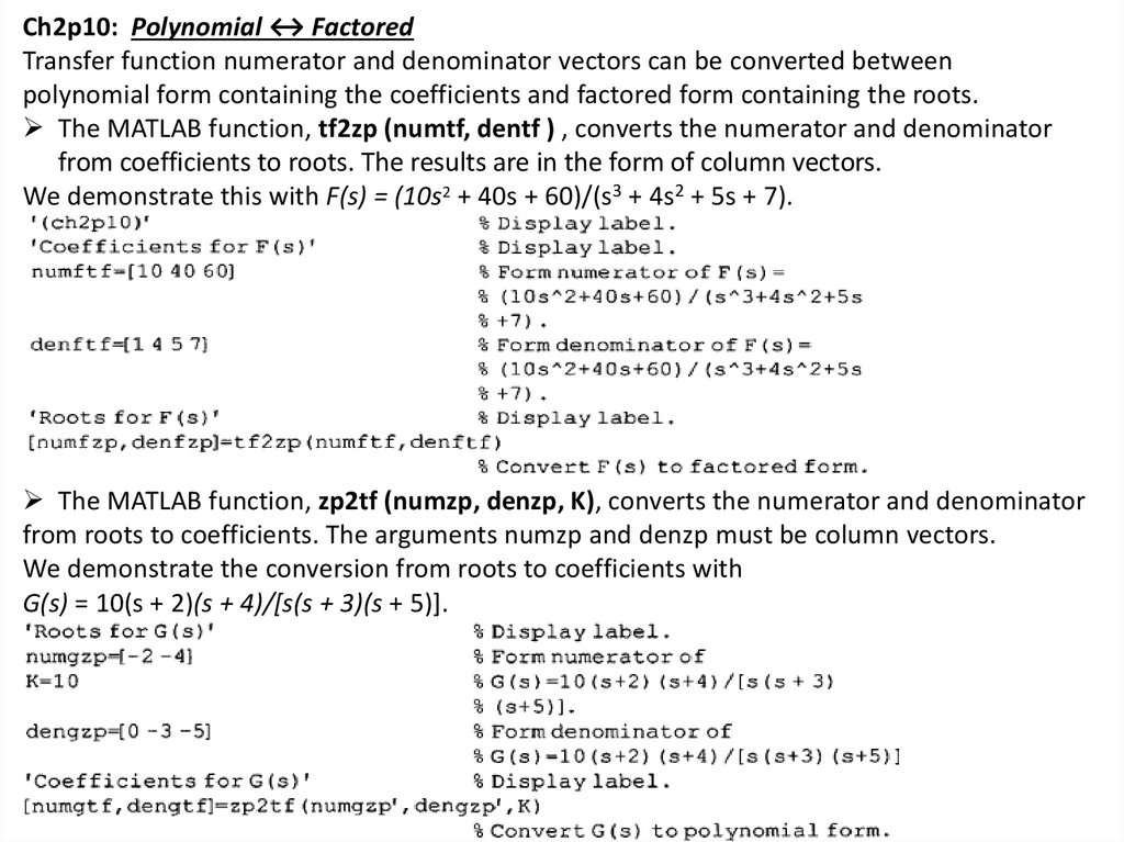
Ch2p10: Polynomial ↔ FactoredTransfer function numerator and denominator vectors can be converted between
polynomial form containing the coefficients and factored form containing the roots.
The MATLAB function, tf2zp (numtf, dentf ) , converts the numerator and denominator
from coefficients to roots. The results are in the form of column vectors.
We demonstrate this with F(s) = (10s2 + 40s + 60)/(s3 + 4s2 + 5s + 7).
The MATLAB function, zp2tf (numzp, denzp, K), converts the numerator and denominator
from roots to coefficients. The arguments numzp and denzp must be column vectors.
We demonstrate the conversion from roots to coefficients with
G(s) = 10(s + 2)(s + 4)/[s(s + 3)(s + 5)].
9.
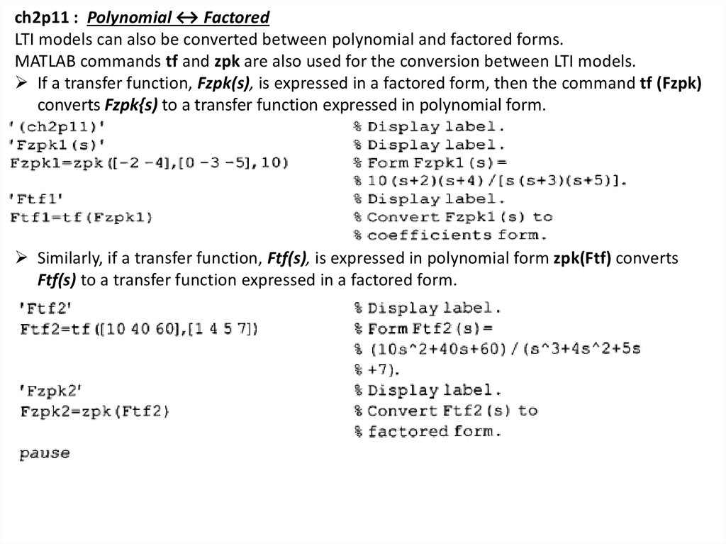
ch2p11 : Polynomial ↔ FactoredLTI models can also be converted between polynomial and factored forms.
MATLAB commands tf and zpk are also used for the conversion between LTI models.
If a transfer function, Fzpk(s), is expressed in a factored form, then the command tf (Fzpk)
converts Fzpk{s) to a transfer function expressed in polynomial form.
Similarly, if a transfer function, Ftf(s), is expressed in polynomial form zpk(Ftf) converts
Ftf(s) to a transfer function expressed in a factored form.
10.
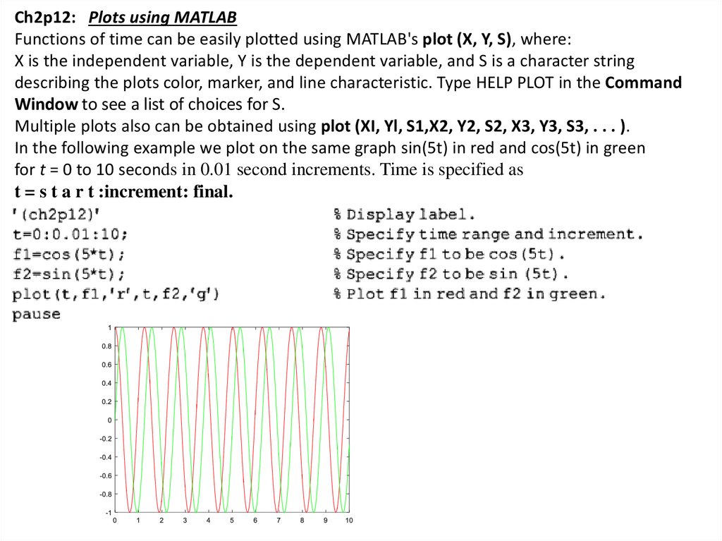
Ch2p12: Plots using MATLABFunctions of time can be easily plotted using MATLAB's plot (X, Y, S), where:
X is the independent variable, Y is the dependent variable, and S is a character string
describing the plots color, marker, and line characteristic. Type HELP PLOT in the Command
Window to see a list of choices for S.
Multiple plots also can be obtained using plot (XI, Yl, S1,X2, Y2, S2, X3, Y3, S3, . . . ).
In the following example we plot on the same graph sin(5t) in red and cos(5t) in green
for t = 0 to 10 seconds in 0.01 second increments. Time is specified as
t = s t a r t :increment: final.