Introduction to R programming. Practical class #2

1.

INTRODUCTION TO R PROGRAMMING
MASTER COURSE FOR SPECIALTY 1-31 80 01 BIOLOGY
Practical class #2.
Vasily V. Grinev
Ph.D., Associate Professor
Department of Genetics
Faculty of Biology
Belarusian State University
Minsk
Republic of Belarus

2.

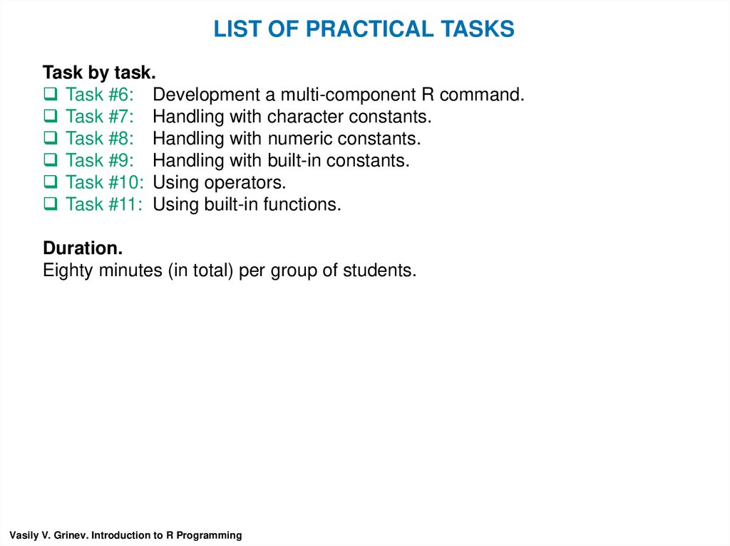
LIST OF PRACTICAL TASKS
Task by task.
Task #6: Development a multi-component R command.
Task #7: Handling with character constants.
Task #8: Handling with numeric constants.
Task #9: Handling with built-in constants.
Task #10: Using operators.
Task #11: Using built-in functions.
Duration.
Eighty minutes (in total) per group of students.
Vasily V. Grinev. Introduction to R Programming

3.

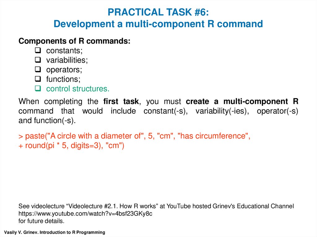
PRACTICAL TASK #6:
Development a multi-component R command
Components of R commands:
constants;
variabilities;
operators;
functions;
control structures.
When completing the first task, you must create a multi-component R
command that would include constant(-s), variability(-ies), operator(-s)
and function(-s).
> paste("A circle with a diameter of", 5, "cm", "has circumference",
+ round(pi * 5, digits=3), "cm")
See videolecture “Videolecture #2.1. How R works” at YouTube hosted Grinev's Educational Channel
https://www.youtube.com/watch?v=4bsf23GKy8c
for future details.
Vasily V. Grinev. Introduction to R Programming

4.

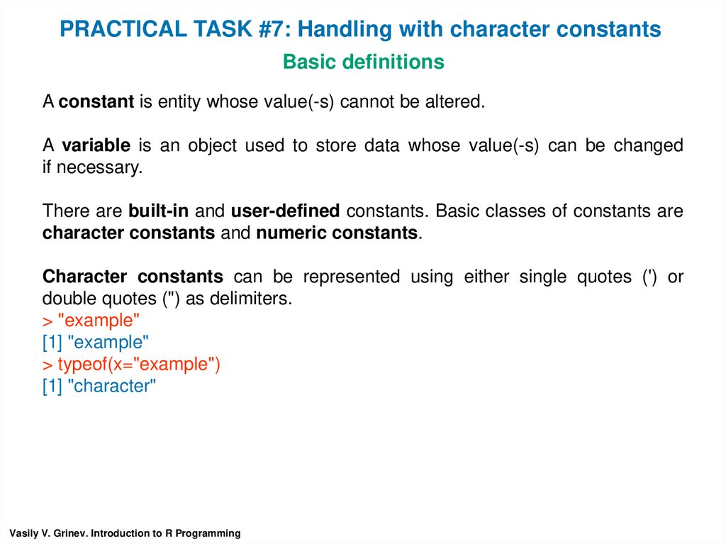
PRACTICAL TASK #7: Handling with character constants
Basic definitions
A constant is entity whose value(-s) cannot be altered.
A variable is an object used to store data whose value(-s) can be changed
if necessary.
There are built-in and user-defined constants. Basic classes of constants are
character constants and numeric constants.
Character constants can be represented using either single quotes (') or
double quotes (") as delimiters.
> "example"
[1] "example"
> typeof(x="example")
[1] "character"
Vasily V. Grinev. Introduction to R Programming

5.

PRACTICAL TASK #7: Handling with character constants
Task content
Creating a character constant:
> "example"
[1] "example“
> con <- "example"
> con
[1] "example"
Replacement of constant:
> con1 <- "blood"
> con1
[1] "blood"
> con2 <- sub(pattern="loo", replacement="rea", x=con1)
> con2
[1] "bread"
Vasily V. Grinev. Introduction to R Programming

6.

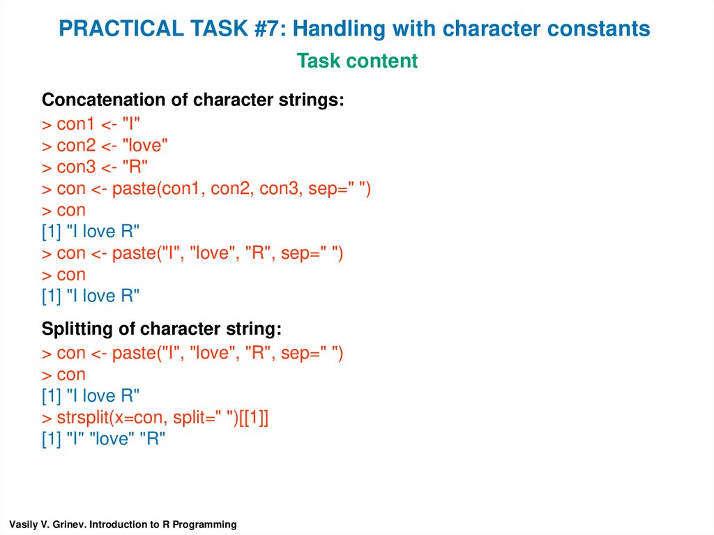
PRACTICAL TASK #7: Handling with character constants
Task content
Concatenation of character strings:
> con1 <- "I"
> con2 <- "love"
> con3 <- "R"
> con <- paste(con1, con2, con3, sep=" ")
> con
[1] "I love R"
> con <- paste("I", "love", "R", sep=" ")
> con
[1] "I love R"
Splitting of character string:
> con <- paste("I", "love", "R", sep=" ")
> con
[1] "I love R"
> strsplit(x=con, split=" ")[[1]]
[1] "I" "love" "R"
Vasily V. Grinev. Introduction to R Programming

7.

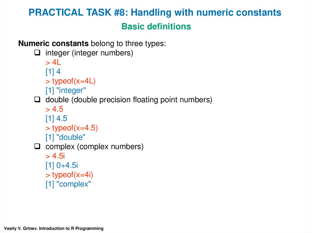
PRACTICAL TASK #8: Handling with numeric constants
Basic definitions
Numeric constants belong to three types:
integer (integer numbers)
> 4L
[1] 4
> typeof(x=4L)
[1] "integer"
double (double precision floating point numbers)
> 4.5
[1] 4.5
> typeof(x=4.5)
[1] "double"
complex (complex numbers)
> 4.5i
[1] 0+4.5i
> typeof(x=4i)
[1] "complex"
Vasily V. Grinev. Introduction to R Programming

8.

PRACTICAL TASK #8: Handling with numeric constants
Task content
Creating an integer constant:
### by appending an L suffix
> con <- 5L
> con
[1] 5
### by function as.integer()
> con <- as.integer(x=5)
> con
[1] 5
> as.integer(x=5.4)
[1] 5
> as.integer(x="5.4")
[1] 5
> as.integer(x="love")
[1] NA
Warning message:
NAs introduced by coercion
Vasily V. Grinev. Introduction to R Programming

9.

PRACTICAL TASK #8: Handling with numeric constants
Task content
Inspection a type and/or class of integer constant:
> con <- 5L
### by function typeof()
> typeof(x=con)
[1] "integer"
### by function class()
> class(x=con)
[1] "integer“
### by function is.integer()
> is.integer(x=con)
[1] TRUE
Vasily V. Grinev. Introduction to R Programming

10.

PRACTICAL TASK #8: Handling with numeric constants
Task content
The reasons for existing integer constants:
The integer is represented explicitly. At the same time, the representing real numbers
always involves an approximation and a potential loss of significant digits.
Testing for the equality of two real numbers is not a realistic way to think when dealing
with the numbers in a computer. Direct comparison of real numbers can cause errors.
Performing arithmetic on very small or very large real numbers can lead to errors that
are not possible in abstract mathematics.
The more bits we use to represent a real number, the greater the precision of the
representation and the more memory we consume.
### memory allocation
> object.size(x=1:100)
448 bytes
> object.size(x=as.numeric(x=1:100))
848 bytes
Vasily V. Grinev. Introduction to R Programming

11.

PRACTICAL TASK #9: Handling with built-in constants
Basic definitions
There are several built-in constants:
The 26 upper-case letters of the Roman alphabet
> LETTERS
[1] "A" "B" "C" "D" "E" "F" "G" "H" "I" "J" "K" "L" "M" "N" "O" "P" "Q"
[18] "R" "S" "T" "U" "V" "W" "X" "Y" "Z"
The 26 lower-case letters of the Roman alphabet
> letters
[1] "a" "b" "c" "d" "e" "f" "g" "h" "i" "j" "k" "l" "m" "n" "o" "p" "q" "r" "s" "t"
[21] "u" "v" "w" "x" "y" "z"
The English names for the months of the year
> month.name
[1] "January" "February" "March" "April" "May" "June" "July" "August"
[9] "September" "October" "November" "December"
The three-letter abbreviations for the English month names
> month.abb
[1] "Jan" "Feb" "Mar" "Apr" "May" "Jun" "Jul" "Aug" "Sep" "Oct"
[11] "Nov" "Dec"
The ratio of the circumference of a circle to its diameter
> pi
[1] 3.141593
Vasily V. Grinev. Introduction to R Programming

12.

PRACTICAL TASK #9: Handling with built-in constants
Task content
Some manipulations with character built-in constants:
> LETTERS
[1] "A" "B" "C" "D" "E" "F" "G" "H" "I" "J" "K" "L" "M" "N" "O" "P" "Q" "R" "S" "T"
[20] "T" "U" "V" "W" "X" "Y" "Z"
> tolower(x=LETTERS)
[1] "a" "b" "c" "d" "e" "f" "g" "h" "i" "j" "k" "l" "m" "n" "o" "p" "q" "r" "s" "t" "u" "v“
[23] "w" "x" "y" "z"
> toupper(x=letters)
[1] "A" "B" "C" "D" "E" "F" "G" "H" "I" "J" "K" "L" "M" "N" "O" "P" "Q" "R" "S" "T"
[20] "T" "U" "V" "W" "X" "Y" "Z"
> month.name
[1] "January" "February" "March" "April" "May" "June" "July" "August"
[9] "September" "October" "November" "December“
> substr(x=month.name, start=1, stop=3)
[1] "Jan" "Feb" "Mar" "Apr" "May" "Jun" "Jul" "Aug" "Sep" "Oct" "Nov" "Dec"
Vasily V. Grinev. Introduction to R Programming

13.

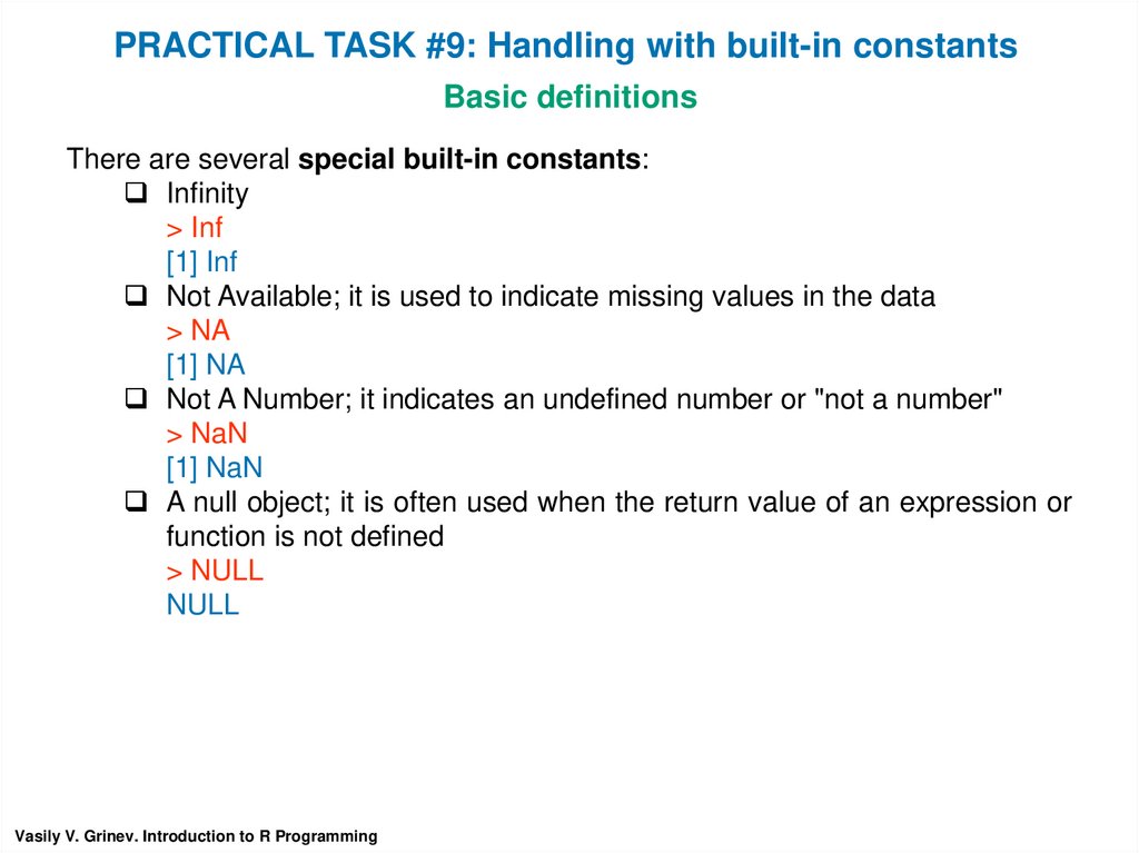
PRACTICAL TASK #9: Handling with built-in constants
Basic definitions
There are several special built-in constants:
Infinity
> Inf
[1] Inf
Not Available; it is used to indicate missing values in the data
> NA
[1] NA
Not A Number; it indicates an undefined number or "not a number"
> NaN
[1] NaN
A null object; it is often used when the return value of an expression or
function is not defined
> NULL
NULL
Vasily V. Grinev. Introduction to R Programming

14.

PRACTICAL TASK #9: Handling with built-in constants
Task content
Some manipulations with special built-in constants:
> v <- 4:13
>v
[1] 4 5 6 7 8 9 10 11 12 13
> v[c(2, 4, 7)] <- c(5/0, NA, NaN)
>v
[1] 4 Inf 6 NA 8 9 NaN 11 12 13
> is.na(x=v)
[1] FALSE FALSE FALSE TRUE FALSE FALSE TRUE FALSE FALSE FALSE
> is.nan(x=v)
[1] FALSE FALSE FALSE FALSE FALSE FALSE TRUE FALSE FALSE FALSE
> is.finite(x=v)
[1] TRUE FALSE TRUE FALSE TRUE TRUE FALSE TRUE TRUE TRUE
> is.infinite(x=v)
[1] FALSE TRUE FALSE FALSE FALSE FALSE FALSE FALSE FALSE FALSE
> table(is.infinite(v))
FALSE TRUE
9
1
Vasily V. Grinev. Introduction to R Programming

15.

PRACTICAL TASK #10: Using operators
Basic definitions
In any programming language, an operator is a symbol that tells the compiler
or interpreter to perform specific operation and produce final result.
Type (category) of operators in R:
arithmetic operators;
relational operators;
logical operators;
assignment operators;
miscellaneous operators.
You can get help about any operator via ?"operator_name".
For future reading:
1) Operator (computer programming) (https://en.wikipedia.org/wiki/Operator_(computer_programming))
2) Basics of operators (https://www.hackerearth.com/ru/practice/basic-programming/operators)
3) R operators (https://www.datamentor.io/r-programming/operator)
4) R-operators (https://www.tutorialspoint.com/r/r_operators.htm)
5) Operators in C/C++ (https://www.geeksforgeeks.org/operators-c-c/)
6) Java - Basic operators (https://www.tutorialspoint.com/java/java_basic_operators.htm)
Vasily V. Grinev. Introduction to R Programming

16.

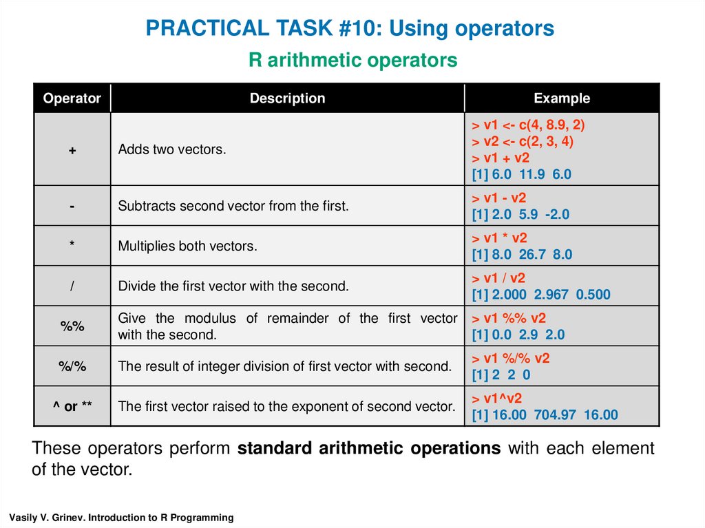
PRACTICAL TASK #10: Using operators
R arithmetic operators
Operator
Description
Example
+
Adds two vectors.
> v1 <- c(4, 8.9, 2)
> v2 <- c(2, 3, 4)
> v1 + v2
[1] 6.0 11.9 6.0
-
Subtracts second vector from the first.
> v1 - v2
[1] 2.0 5.9 -2.0
*
Multiplies both vectors.
> v1 * v2
[1] 8.0 26.7 8.0
/
Divide the first vector with the second.
> v1 / v2
[1] 2.000 2.967 0.500
%%
Give the modulus of remainder of the first vector
with the second.
> v1 %% v2
[1] 0.0 2.9 2.0
%/%
The result of integer division of first vector with second.
> v1 %/% v2
[1] 2 2 0
^ or **
The first vector raised to the exponent of second vector.
> v1^v2
[1] 16.00 704.97 16.00
These operators perform standard arithmetic operations with each element
of the vector.
Vasily V. Grinev. Introduction to R Programming

17.

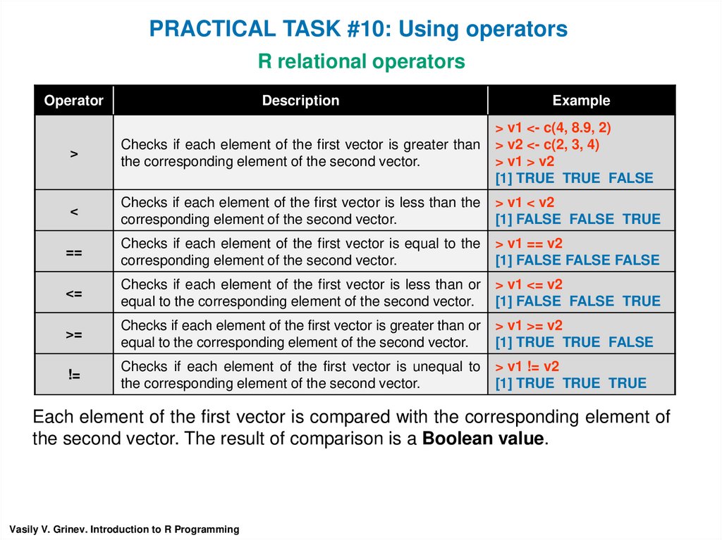
PRACTICAL TASK #10: Using operators
R relational operators
Operator
Description
Example
>
Checks if each element of the first vector is greater than
the corresponding element of the second vector.
> v1 <- c(4, 8.9, 2)
> v2 <- c(2, 3, 4)
> v1 > v2
[1] TRUE TRUE FALSE
<
Checks if each element of the first vector is less than the
corresponding element of the second vector.
> v1 < v2
[1] FALSE FALSE TRUE
==
Checks if each element of the first vector is equal to the
corresponding element of the second vector.
> v1 == v2
[1] FALSE FALSE FALSE
<=
Checks if each element of the first vector is less than or
equal to the corresponding element of the second vector.
> v1 <= v2
[1] FALSE FALSE TRUE
>=
Checks if each element of the first vector is greater than or
equal to the corresponding element of the second vector.
> v1 >= v2
[1] TRUE TRUE FALSE
!=
Checks if each element of the first vector is unequal to
the corresponding element of the second vector.
> v1 != v2
[1] TRUE TRUE TRUE
Each element of the first vector is compared with the corresponding element of
the second vector. The result of comparison is a Boolean value.
Vasily V. Grinev. Introduction to R Programming

18.

PRACTICAL TASK #10: Using operators
R logical operators
Operator
Description
Example
!
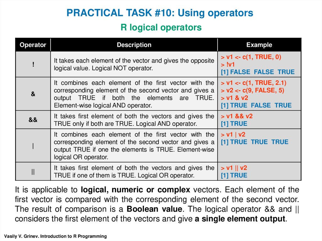
It takes each element of the vector and gives the opposite
logical value. Logical NOT operator.
> v1 <- c(1, TRUE, 0)
> !v1
[1] FALSE FALSE TRUE
&
It combines each element of the first vector with the
corresponding element of the second vector and gives a
output TRUE if both the elements are TRUE.
Element-wise logical AND operator.
> v1 <- c(1, TRUE, 2.1)
> v2 <- c(9, FALSE, 5)
> v1 & v2
[1] TRUE FALSE TRUE
&&
It takes first element of both the vectors and gives the
TRUE only if both are TRUE. Logical AND operator.
> v1 && v2
[1] TRUE
|
It combines each element of the first vector with the
corresponding element of the second vector and gives a
output TRUE if one the elements is TRUE. Element-wise
logical OR operator.
> v1 | v2
[1] TRUE TRUE TRUE
||
It takes first element of both the vectors and gives the
TRUE if one of them is TRUE. Logical OR operator.
> v1 || v2
[1] TRUE
It is applicable to logical, numeric or complex vectors. Each element of the
first vector is compared with the corresponding element of the second vector.
The result of comparison is a Boolean value. The logical operator && and ||
considers the first element of the vectors and give a single element output.
Vasily V. Grinev. Introduction to R Programming

19.

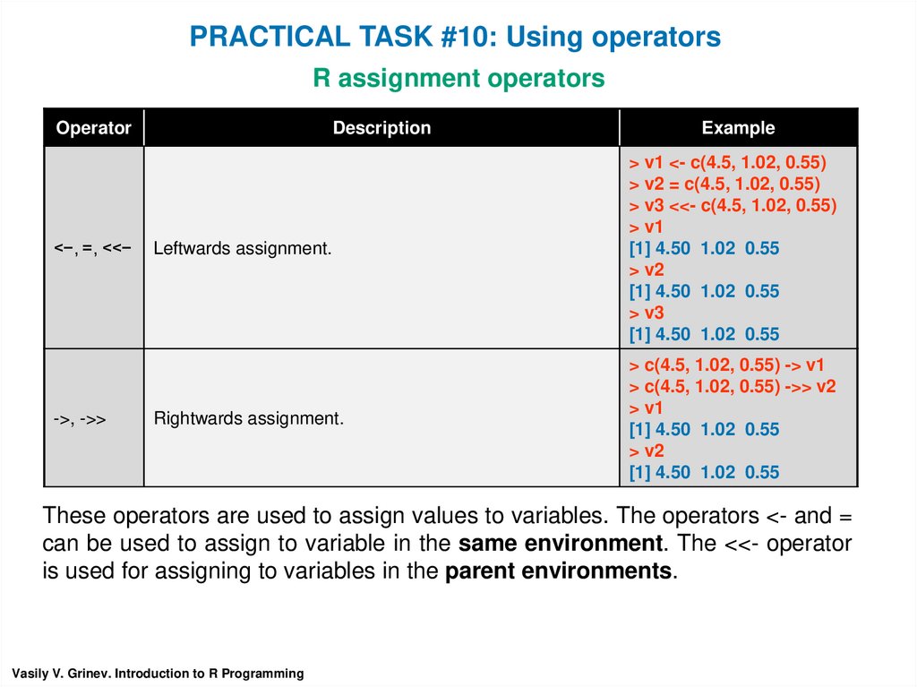
PRACTICAL TASK #10: Using operators
R assignment operators
Operator
<−, =, <<−
->, ->>
Description
Example
Leftwards assignment.
> v1 <- c(4.5, 1.02, 0.55)
> v2 = c(4.5, 1.02, 0.55)
> v3 <<- c(4.5, 1.02, 0.55)
> v1
[1] 4.50 1.02 0.55
> v2
[1] 4.50 1.02 0.55
> v3
[1] 4.50 1.02 0.55
Rightwards assignment.
> c(4.5, 1.02, 0.55) -> v1
> c(4.5, 1.02, 0.55) ->> v2
> v1
[1] 4.50 1.02 0.55
> v2
[1] 4.50 1.02 0.55
These operators are used to assign values to variables. The operators <- and =
can be used to assign to variable in the same environment. The <<- operator
is used for assigning to variables in the parent environments.
Vasily V. Grinev. Introduction to R Programming

20.

PRACTICAL TASK #10: Using operators
R miscellaneous operators
Operator
Description
:
It creates the series of numbers in sequence for
a vector.
> v1 <- 4:9
> v1
[1] 4 5 6 7 8 9
This operator is used to identify if an element
(or elements) belongs to a vector.
> v1 <- 4:9
> v2 <- c(7, 10)
> v2 %in% v1
[1] TRUE FALSE
This operator is used to multiply a matrix.
> m <- matrix(data=c(2, 6, 1, 5),
nrow=2,
ncol=2,
byrow=TRUE)
>m
[,1] [,2]
[1,]
2
6
[2,]
1
5
> m %*% m
[,1] [,2]
[1,] 10 42
[2,]
7 31
%in%
%*%
Example
These operators are used for specific purposes and not general arithmetic or
logical computation.
Vasily V. Grinev. Introduction to R Programming

21.

PRACTICAL TASK #10: Using operators
R miscellaneous operators
Operator
Description
'…', "…"
Single or double quotes are used to create an
object of type character.
> v1 <- "Hi everyone!"
> v1
[1] "Hi everyone!"
#
It is a comment operator. Everything to the right
of the operator is treated as a comment.
> v1 <- 4:9 #3:19
> v1
[1] 4 5 6 7 8 9
It separates expressions in one line.
> c(1, 2); 2 + 3
[1] 1 2
[1] 5
;
Vasily V. Grinev. Introduction to R Programming
Example

22.

PRACTICAL TASK #10: Using operators
Task content
Practice with all main R operators. Use the true data sets.
> v <- 4:13
>v
[1] 4 5 6 7 8 9 10 11 12 13
>v+1
[1] 5 6 7 8 9 10 11 12 13 14
Vasily V. Grinev. Introduction to R Programming

23.

PRACTICAL TASK #11: Using built-in functions
Basic definitions
Built-in function is a function which already created or defined in the
programming framework.
Built-in functions in R:
math, or numeric, functions;
character, or string, functions;
basic statistical functions;
statistical probability functions;
other functions.
You can get help about any built-in function via ?function_name.
See videolecture “Videolecture #9.1. Introduction in R functions” at YouTube hosted Grinev's
Educational Channel https://www.youtube.com/watch?v=Lf-B4fNXm1g&t=696s
for future details.
Vasily V. Grinev. Introduction to R Programming

24.

PRACTICAL TASK #11: Using built-in functions
R math functions
Function
Description
Example
abs()
It returns the absolute value of input x.
> abs(x=-10.1)
[1] 10.1
sqrt()
It returns the square root of input x.
> sqrt(x=12)
[1] 3.464102
ceiling()
It returns the smallest integer which is larger than
or equal to x.
> ceiling(x=4.6)
[1] 5
floor()
It returns the largest integer, which is smaller than
or equal to x.
> floor(x=2.9)
[1] 2
trunc()
It returns the truncate value of input x.
> trunc(x=c(1.2, 3.4, 5.6))
[1] 1 3 5
round()
It returns round value of input x.
> round(x=c(1.2, 3.4, 5.6))
[1] 1 3 7
It returns cos, sin or tan value of input x.
> cos(x=10)
[1] -0.8390715
log()
It returns natural logarithm of input x.
> log(x=45, base=exp(1))
[1] 3.806662
exp()
It returns exponent.
> exp(x=15)
[1] 3269017
cos(), sin(), tan()
Vasily V. Grinev. Introduction to R Programming

25.

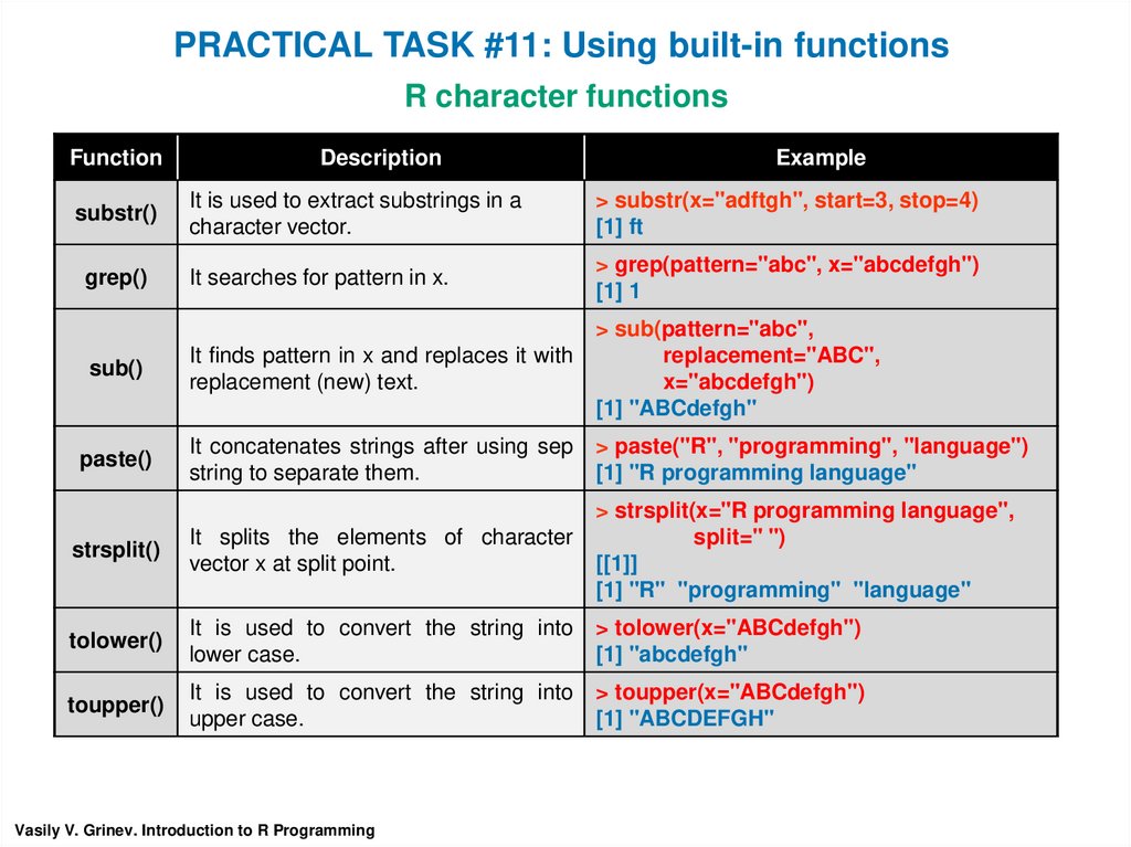
PRACTICAL TASK #11: Using built-in functions
R character functions
Function
Description
Example
substr()
It is used to extract substrings in a
character vector.
> substr(x="adftgh", start=3, stop=4)
[1] ft
grep()
It searches for pattern in x.
> grep(pattern="abc", x="abcdefgh")
[1] 1
sub()
It finds pattern in x and replaces it with
replacement (new) text.
> sub(pattern="abc",
replacement="ABC",
x="abcdefgh")
[1] "ABCdefgh"
paste()
It concatenates strings after using sep
string to separate them.
> paste("R", "programming", "language")
[1] "R programming language"
strsplit()
It splits the elements of character
vector x at split point.
> strsplit(x="R programming language",
split=" ")
[[1]]
[1] "R" "programming" "language"
tolower()
It is used to convert the string into
lower case.
> tolower(x="ABCdefgh")
[1] "abcdefgh"
toupper()
It is used to convert the string into
upper case.
> toupper(x="ABCdefgh")
[1] "ABCDEFGH"
Vasily V. Grinev. Introduction to R Programming

26.

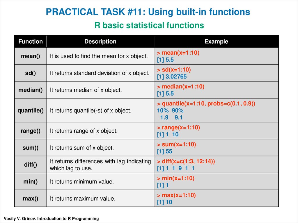
PRACTICAL TASK #11: Using built-in functions
R basic statistical functions
Function
Description
mean()
It is used to find the mean for x object.
> mean(x=1:10)
[1] 5.5
sd()
It returns standard deviation of x object.
> sd(x=1:10)
[1] 3.02765
It returns median of x object.
> median(x=1:10)
[1] 5.5
quantile()
It returns quantile(-s) of x object.
> quantile(x=1:10, probs=c(0.1, 0.9))
10% 90%
1.9 9.1
range()
It returns range of x object.
> range(x=1:10)
[1] 1 10
sum()
It returns sum of x object.
> sum(x=1:10)
[1] 55
diff()
It returns differences with lag indicating
which lag to use.
> diff(x=c(1:3, 12:14))
[1] 1 1 9 1 1
min()
It returns minimum value.
> min(x=1:10)
[1] 1
max()
It returns maximum value.
> max(x=1:10)
[1] 10
median()
Vasily V. Grinev. Introduction to R Programming
Example

27.

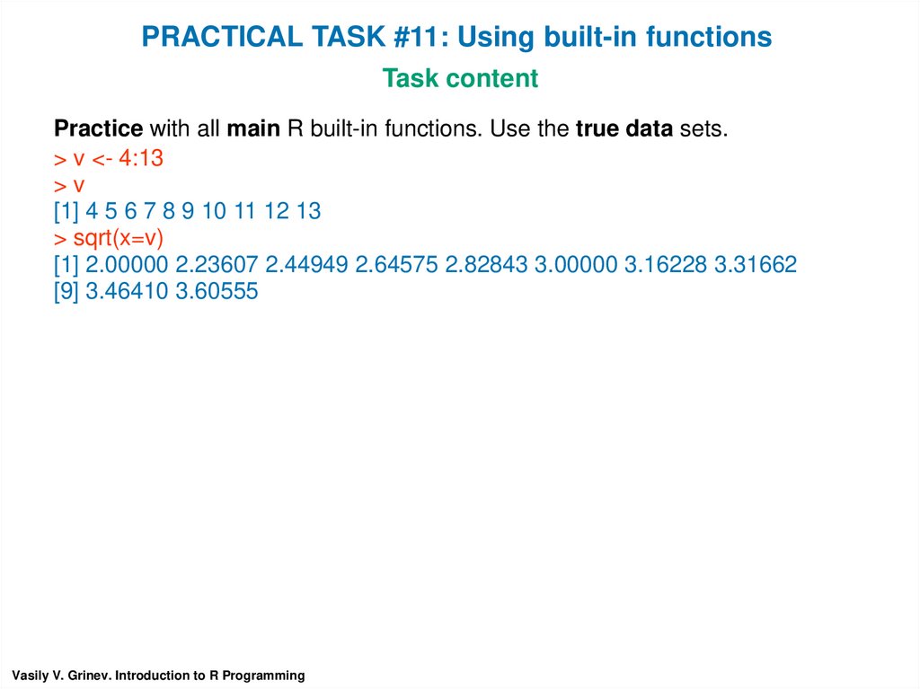
PRACTICAL TASK #11: Using built-in functions
Task content
Practice with all main R built-in functions. Use the true data sets.
> v <- 4:13
>v
[1] 4 5 6 7 8 9 10 11 12 13
> sqrt(x=v)
[1] 2.00000 2.23607 2.44949 2.64575 2.82843 3.00000 3.16228 3.31662
[9] 3.46410 3.60555
Vasily V. Grinev. Introduction to R Programming

28.

THANKS FOR YOUR ATTENTION!
https://www.sr-sv.com/the-power-of-r-for-trading-part-1/