


 Программирование
 Базы данных
Похожие презентации:


Types and basic structures data in R
1.
Types and basic structures data in R2.
The purpose of the lecture is to familiarize yourself with the basic data typesused in the R language, as well as with the basic structures that the R language
operates on.
As a result of studying the lecture materials, you will know how to create data
of various types, as well as operate on the main data structures.
Statistical programming languages
2
3.
Lecture questions1. Data types in R
2. Basic data structures:
2.1 Vectors
2.2 Matrices
2.3 Arrays
2.4 Frames
2.5 Factors
2.6 Lists
Statistical programming languages
3
4.
Literary source :1.
2.
3.
Visual statistics. We use R! A. B. Shipunov, E. M. Baldin, P. A. Volkova, A. I.
Korobeinikov, S. A. Nazarova, S. V. Petrov, V. G. Sufiyanov. 2014 year
Introduction to R: Notes on R: a programming environment for analyzing data
and graphics. Version 3.1.0 (2014-04-10) U.N. Venables, D.M. Smith.,
Translation from English. - Moscow, 2014.109 s. - (series of technical
documentation).
Statistical analysis and data visualization using R. S.E. Mastitsky, V.K. Shitikov,
Heidelberg - London - Tolyatti, 2014.401 p. Website: http://ranalytics.blogspot.co Website: http://www.qsar4u.com/files/rintro/01.html
Statistical programming languages
4
5.
2. Data Types in RStructured and unstructured
Clean and dirty
Numerical, classification
Symbols, text, pictures, speech
80% of the work is collecting and cleaning data !
Big data is usually BIG and unstructured
Statistical programming languages
5
6.
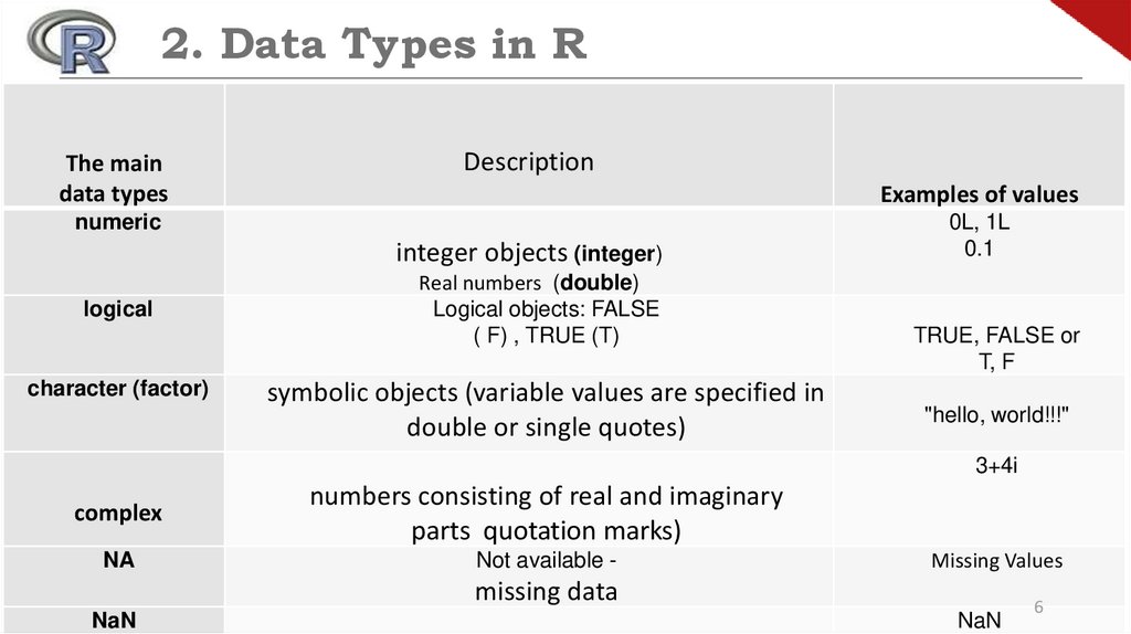
2. Data Types in RThe main
data types
Description
Examples of values
numeric
integer objects (integer)
logical
character (factor)
Real numbers (double)
Logical objects: FALSE
( F) , TRUE (T)
symbolic objects (variable values are specified in
double or single quotes)
0L, 1L
0.1
TRUE, FALSE or
T, F
"hello, world!!!"
3+4i
сomplex
numbers consisting of real and imaginary
parts quotation marks)
NA
Not available -
Missing Values
missing data
NaN
Statistical programming languages
NaN
6
7.
2. Data Types in R• Retrieving Data Type Information :
>class (x)
• Type Verification :
>class(present$year)
[1] "numeric"
>is.[type] (x)
>is.logical(present$year)
[1] FALSE
>is.list(x)
• Type cast :
>as.factor(present$year)
>as.[type] (x)
>as. numeric(x)
[1] 1940 1941 1942 1943 1944 1945 1946 1947 1948 1949 1950 1951 1952 1953
1954 [16] 1955 1956 1957 1958 1959 1960 1961 1962 1963 1964 1965 1966
1967 1968 1969 [31] 1970 1971 1972 1973 1974 1975 1976 1977 1978 1979
1980 1981 1982 1983 1984 [46] 1985 1986 1987 1988 1989 1990 1991 1992
1993 1994 1995 1996 1997 1998 1999 [61] 2000 2001 2002
63 Levels: 1940 1941 1942 1943 1944 1945 1946 1947 1948 1949 1950 1951
... 2002
Statistical programming languages
7
8.
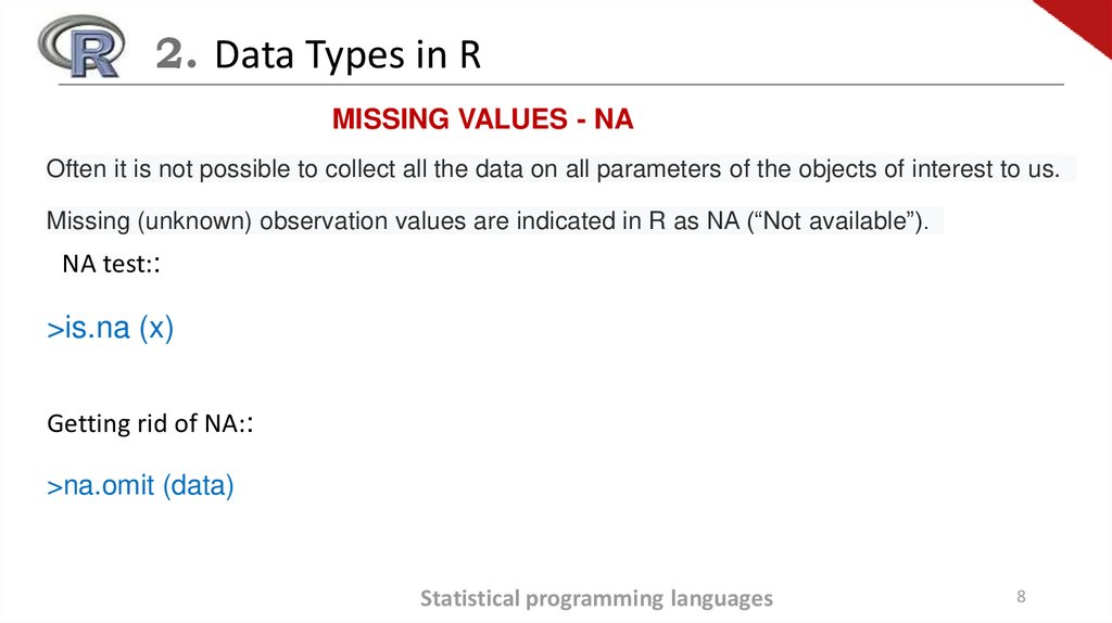
2. Data Types in RMISSING VALUES - NA
Often it is not possible to collect all the data on all parameters of the objects of interest to us.
Missing (unknown) observation values are indicated in R as NA (“Not available”).
NA test::
>is.na (x)
Getting rid of NA::
>na.omit (data)
Statistical programming languages
8
9.
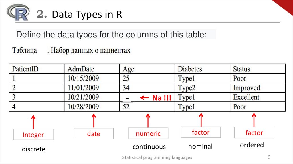
2. Data Types in RDefine the data types for the columns of this table:
−
Integer
discrete
date
Na !!!
numeric
factor
continuous
nominal
Statistical programming languages
factor
ordered
9
10.
3. Basic data structuresStatistical programming languages
10
11.
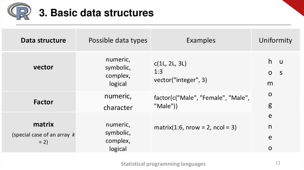
3. Basic data structuresData structure
vector
Factor
matrix
(special case of an array k
= 2)
Possible data types
numeric,
symbolic,
complex,
logical
numeric,
character
numeric,
symbolic,
complex,
logical
Examples
с(1L, 2L, 3L)
1:3
vector("integer", 3)
factor(c("Male", "Female", "Male",
"Male"))
matrix(1:6, nrow = 2, ncol = 3)
Statistical programming languages
Uniformity
h u
o s
m
o
g
e
n
e
o
11
12.
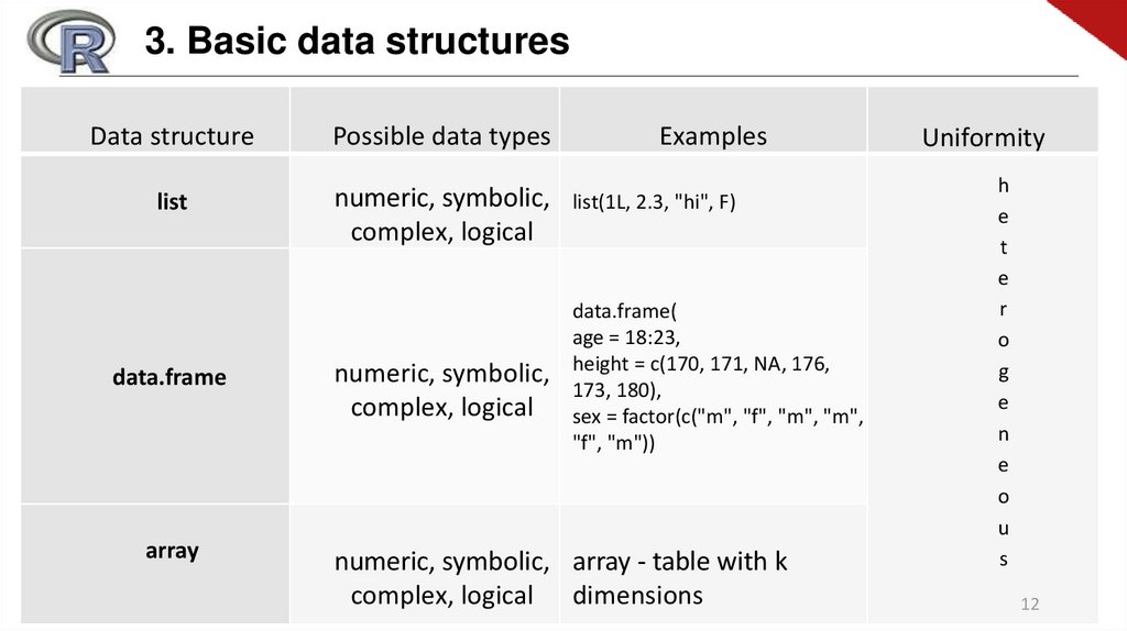
3. Basic data structuresData structure
Possible data types
list
numeric, symbolic,
complex, logical
data.frame
array
numeric, symbolic,
complex, logical
Examples
list(1L, 2.3, "hi", F)
data.frame(
age = 18:23,
height = c(170, 171, NA, 176,
173, 180),
sex = factor(c("m", "f", "m", "m",
"f", "m"))
numeric, symbolic, array - table with k
complex, logical dimensions
Statistical programming languages
Uniformity
h
e
t
e
r
o
g
e
n
e
o
u
s
12
13.
3. Features of the data structure in Ran R object is everything that can be represented in the form of variables, including
constants, various data types, functions, and even diagrams.
Objects have: view (determines in what form the object is stored in memory) and a class
(which tells common functions of type print how to handle it).
A data frame is a type of data structure in R that is similar to the type in which
data is stored in ordinary statistical programs (in SAS, SPSS and STATA).
Columns are variables, and rows are observations. Variable types of variables can be
contained in one data table. Data tables are the main type of data structure.
Factors are nominal or ordinal variables. In R, they are stored and processed in a special way.
Statistical programming languages
13
14.
3. Basic data structures: vectorsVectors are vector data arrays that can contain numeric, textual, or logical data. To create a
vector, the union function c () is used.:
a <- c(1, 2, 5, 3, 6, -2, 4)
b <- c("one", "two", "three")
c <- c(TRUE, TRUE, TRUE, FALSE, TRUE, FALSE)
Statistical programming languages
14
15.
3. Basic data structures: vectorsIndividual elements of a vector can be called using a numerical vector consisting of element
numbers in square brackets. For example, a [c (2, 4)] denotes the second and fourth
elements of the vector.
a <- c(1, 2, 5, 3, 6, -2, 4)
a[3]
[1] 5
a[c(1, 3, 5)] [1] 1 5 6
a[2:6]
2 5 3 6 -2
The colon in the last example is used to create a sequence of numbers..
a <- c(2:6) is the same as a <- c(2, 3, 4, 5, 6).
Statistical programming languages
15
16.
3. Basic data structures: matricesA matrix is a two-dimensional data array in which each element has the same type (numeric,
textual, or logical). Common format :
mymatrix <- matrix(vector, nrow=number_of_rows, ncol=number_of_columns,
byrow=logical_value, dimnames=list(
char_vector_rownames, char_vector_colnames))
where vector contains elements of the matrix, nrow and ncol define the number of rows and
columns in the matrix, and dimnames contains the names of rows and columns, which are
stored as text vectors (they do not need to be specified). The byrow parameter determines
whether the matrix should be filled by rows (byrow=TRUE) or by columns (by row=FALSE). By
default, the matrix is populated by columns.
Statistical programming languages
16
17.
3. Basic data structures: matricesProgram code. Matrix Creation
y <- matrix(1:20, nrow=5, ncol=4)
y
[,1]
[,2]
[,3]
[1,]
1
6
11
[2,]
2
7
12
[3,]
3
8
13
[4,]
4
9
14
[5,]
5
10
15
[,4]
16
17
18
19
20
Statistical programming languages
17
18.
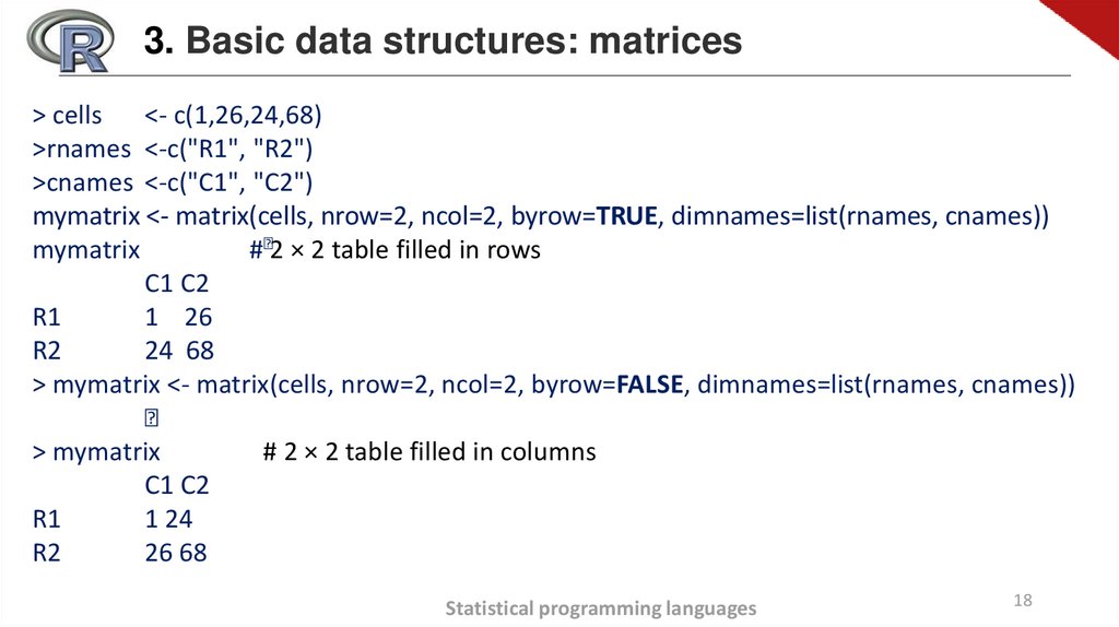
3. Basic data structures: matrices> cells
<- c(1,26,24,68)
>rnames <-c("R1", "R2")
>cnames <-c("C1", "C2")
mymatrix <- matrix(cells, nrow=2, ncol=2, byrow=TRUE, dimnames=list(rnames, cnames))
mymatrix
#2 × 2 table filled in rows
C1 C2
R1
1 26
R2
24 68
> mymatrix <- matrix(cells, nrow=2, ncol=2, byrow=FALSE, dimnames=list(rnames, cnames))
> mymatrix
# 2 × 2 table filled in columns
C1 C2
R1
1 24
R2
26 68
Statistical programming languages
18
19.
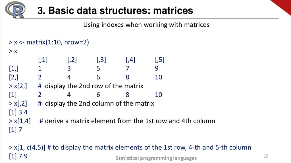
3. Basic data structures: matricesUsing indexes when working with matrices
> x <- matrix(1:10, nrow=2)
>x
[,1]
[,2]
[,3]
[,4]
[,5]
[1,]
1
3
5
7
9
[2,]
2
4
6
8
10
> x[2,] # display the 2nd row of the matrix
[1]
2
4
6
8
10
> x[,2] # display the 2nd column of the matrix
[1] 3 4
> x[1,4] # derive a matrix element from the 1st row and 4th column
[1] 7
> x[1, c(4,5)] # to display the matrix elements of the 1st row, 4-th and 5-th column
[1] 7 9
Statistical programming languages
19
20.
3. Basic data structures: arraysArrays are similar to matrices, but can have more than two dimensions.
myarray <- array(vector, dimensions, dimnames)
where vector contains the data itself, dimensions is a numeric vector specifying the
dimension for each dimension and dimnames is an optional list of dimension
names.
As an example, we give the program code, with the help of which a threedimensional (2×3×4) array of numbers is created.
Statistical programming languages
20
21.
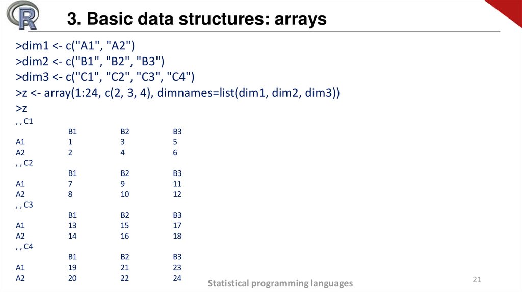
3. Basic data structures: arrays>dim1 <- c("A1", "A2")
>dim2 <- c("B1", "B2", "B3")
>dim3 <- c("C1", "C2", "C3", "C4")
>z <- array(1:24, c(2, 3, 4), dimnames=list(dim1, dim2, dim3))
>z
, , C1
A1
A2
, , C2
A1
A2
, , C3
A1
A2
, , C4
A1
A2
B1
1
2
B2
3
4
B3
5
6
B1
7
8
B2
9
10
B3
11
12
B1
13
14
B2
15
16
B3
17
18
B1
19
20
B2
21
22
B3
23
24
Statistical programming languages
21
22.
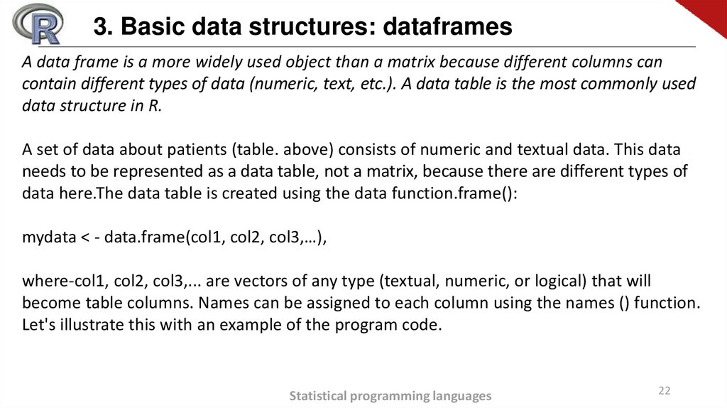
3. Basic data structures: dataframesA data frame is a more widely used object than a matrix because different columns can
contain different types of data (numeric, text, etc.). A data table is the most commonly used
data structure in R.
A set of data about patients (table. above) consists of numeric and textual data. This data
needs to be represented as a data table, not a matrix, because there are different types of
data here.The data table is created using the data function.frame():
mydata < - data.frame(col1, col2, col3,…),
where-col1, col2, col3,... are vectors of any type (textual, numeric, or logical) that will
become table columns. Names can be assigned to each column using the names () function.
Let's illustrate this with an example of the program code.
Statistical programming languages
22
23.
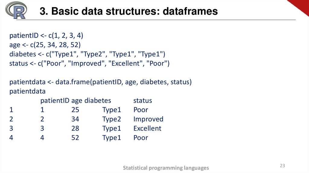
3. Basic data structures: dataframespatientID <- c(1, 2, 3, 4)
age <- c(25, 34, 28, 52)
diabetes <- c("Type1", "Type2", "Type1", "Type1")
status <- c("Poor", "Improved", "Excellent", "Poor")
patientdata <- data.frame(patientID, age, diabetes, status)
patientdata
patientID age diabetes
status
1
1
25
Type1
Poor
2
2
34
Type2
Improved
3
3
28
Type1
Excellent
4
4
52
Type1
Poor
Statistical programming languages
23
24.
3. Basic data structures: dataframesDesignation of data table elements
>patientdata[1:2]
patientID age
1
25
2
34
3
28
4
52
> patientdata[c("diabetes", "status")]
diabetes status
1
Type1
Poor
2
Type2
Improved
3
Type1
Excellent
patientdata$age [1] 25 34 28 52
Statistical programming languages
24
25.
3. Basic data structures: factorsThe factor () function stores categorical data as a vector of integers in the range from one to
k (where k is the number of unique values of the categorical variable) and as an internal
vector of a chain of characters (the original values of the variable) corresponding to these
integers.
diabetes <- c("Type1", "Type2", "Type1", "Type1").
diabetes <- factor(diabetes)
Numeric values are assigned in alphabetical order. Any analysis you do with the diabetes
vector will take this variable as nominal and choose statistical methods that are appropriate
for this type of data.
Statistical programming languages
25
26.
3. Basic data structures: factorsYou can change the default setting by specifying the levels parameter. For example:
>status <- factor(status, order=TRUE,
levels=c("Poor", "Improved", "Excellent"))
will assign levels to the values of the vector as follows:
1=Poor, 2=Improved, 3=Excellent.
Statistical programming languages
26
27.
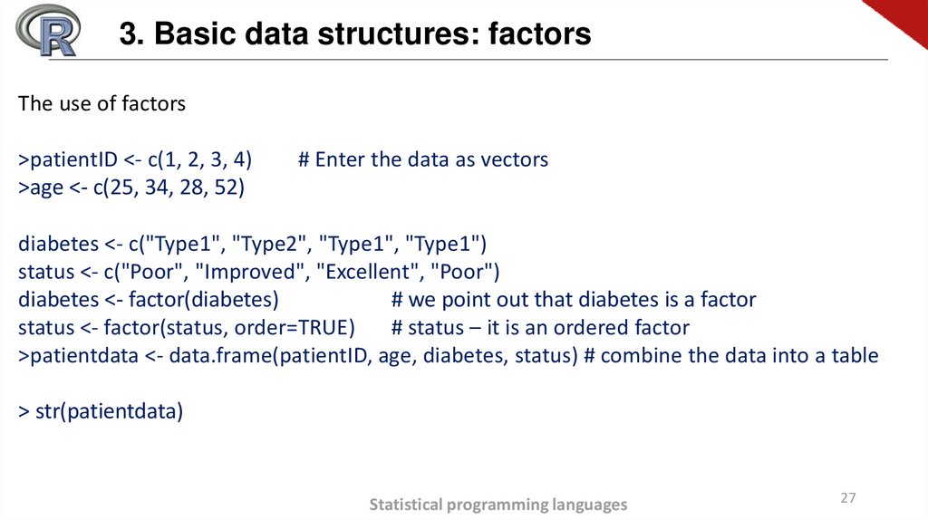
3. Basic data structures: factorsThe use of factors
>patientID <- c(1, 2, 3, 4)
>age <- c(25, 34, 28, 52)
# Enter the data as vectors
diabetes <- c("Type1", "Type2", "Type1", "Type1")
status <- c("Poor", "Improved", "Excellent", "Poor")
diabetes <- factor(diabetes)
# we point out that diabetes is a factor
status <- factor(status, order=TRUE)
# status – it is an ordered factor
>patientdata <- data.frame(patientID, age, diabetes, status) # combine the data into a table
> str(patientdata)
Statistical programming languages
27
28.
3. Basic data structures: listsLists are the most complex data type in R. In fact, a list is an ordered list of objects
(components). For example, a list can be a combination of vectors, matrices, data tables, and
even other lists. The list can be created using the function
list():
mylist <- list(object1, object2, …),
where objects are any data structures we discussed before. Objects in the list can be named:
mylist <- list(name1=object1, name2=object2, …)
Statistical programming languages
28
29.
3. Basic data structures: listsCreating a list
>g <- "My First List"
>h <- c(25, 26, 18, 39)
>j <- matrix(1:10, nrow=5)
>k <- c("one", "two", "three")
> mylist <- list(title=g, ages=h, j, k)
> mylist
mylist[[2]]
> mylist[["ages"]]
# Display the entire list
# Display the second object of the list
# Display the second object of the list
Statistical programming languages
29
30.
Conclusions of the lectureWe
learned:
What data types are used in R
What objects does R operate on
Features of working with basic R structures
Apply arithmetic operators to variables and
vectors
To calculate some statistics with the use of
aggregate functions
Statistical programming languages
30