


 Информатика
Похожие презентации:


")

Developing Efficient Algorithms
1.
Developing EfficientAlgorithms
2.
Objectives▪
▪
▪
▪
▪
▪
▪
▪
▪
▪
▪
▪
▪
▪
To estimate algorithm efficiency using the Big notation (§22.2).
To explain growth rates and why constants and nondominating terms can be ignored in the
estimation (§22.2).
To determine the complexity of various types of algorithms (§22.3).
To analyze the binary search algorithm (§22.4.1).
To analyze the selection sort algorithm (§22.4.2).
To analyze the insertion sort algorithm (§22.4.3).
To analyze the Tower of Hanoi algorithm (§22.4.4).
To describe common growth functions (constant, logarithmic, log-linear, quadratic, cubic,
exponential) (§22.4.5).
To design efficient algorithms for finding Fibonacci numbers using dynamic programming
(§22.5).
To find the GCD using Euclid’s algorithm (§22.6).
To finding prime numbers using the sieve of Eratosthenes (§22.7).
To design efficient algorithms for finding the closest pair of points using the divide-andconquer approach (§22.8).
To solve the Eight Queens problem using the backtracking approach (§22.9).
To design efficient algorithms for finding a convex hull for a set of points (§22.10).
2
3.
IntroductionWhat is algorithm design?
Algorithm design is to develop a mathematical
process for solving a problem.
What is algorithm analysis?
Algorithm analysis is to predict the performance
of an algorithm.
Algorithm executing time is desired to be less.
3
4.
Executing TimeSuppose two algorithms perform the same task such as search
(linear search vs. binary search). Which one is better? One
possible approach to answer this question is to implement these
algorithms in Java and run the programs to get execution time.
But there are two problems for this approach:
▪
▪
First, there are many tasks running concurrently on a computer.
The execution time of a particular program is dependent on the
system load.
Second, the execution time is dependent on specific input.
Consider linear search and binary search for example. If an
element to be searched happens to be the first in the list, linear
search will find the element quicker than binary search.
4
5.
Growth RateIt is very difficult to compare algorithms by measuring
their execution time.
To overcome these problems, a theoretical approach was
developed to analyze algorithms independent of computers
and specific input.
This approach approximates the effect of a change on the
size of the input. In this way, you can see how fast an
algorithm’s execution time increases as the input size
increases, so you can compare two algorithms by
examining their growth rates.
5
6.
Big O NotationConsider linear search. The linear search algorithm compares
the key with the elements in the array sequentially (in order)
until the key is found or all array elements are compared.
If the key is not in the array, it requires n comparisons for an
array of size n. If the key is in the array, it requires n/2
comparisons on average.
The algorithm’s execution time is proportional to the size of the
array. If you double the size of the array, you will expect the
number of comparisons to double.
The algorithm grows at a linear rate. The growth rate has an
order of magnitude of n. The Big O notation is used to
abbreviate for “order of magnitude.” Using this notation, the
complexity of the linear search algorithm is O(n), pronounced as
“order of n.”
6
7.
Best, Worst, and Average CasesFor the same input size, an algorithm’s execution time may vary,
depending on the input.
An input that results in the shortest execution time is called the
best-case input and
an input that results in the longest execution time is called the
worst-case input.
Worst-case analysis is very useful. You can show that the algorithm
will never be slower than the worst-case.
An average-case analysis attempts to determine the average amount
of time among all possible input of the same size. Average-case
analysis is ideal, but difficult to perform, because it is hard to
determine the relative probabilities and distributions of various input
instances for many problems.
Worst-case analysis is easier to obtain and is thus common. So, the
analysis is generally conducted for the worst-case.
7
8.
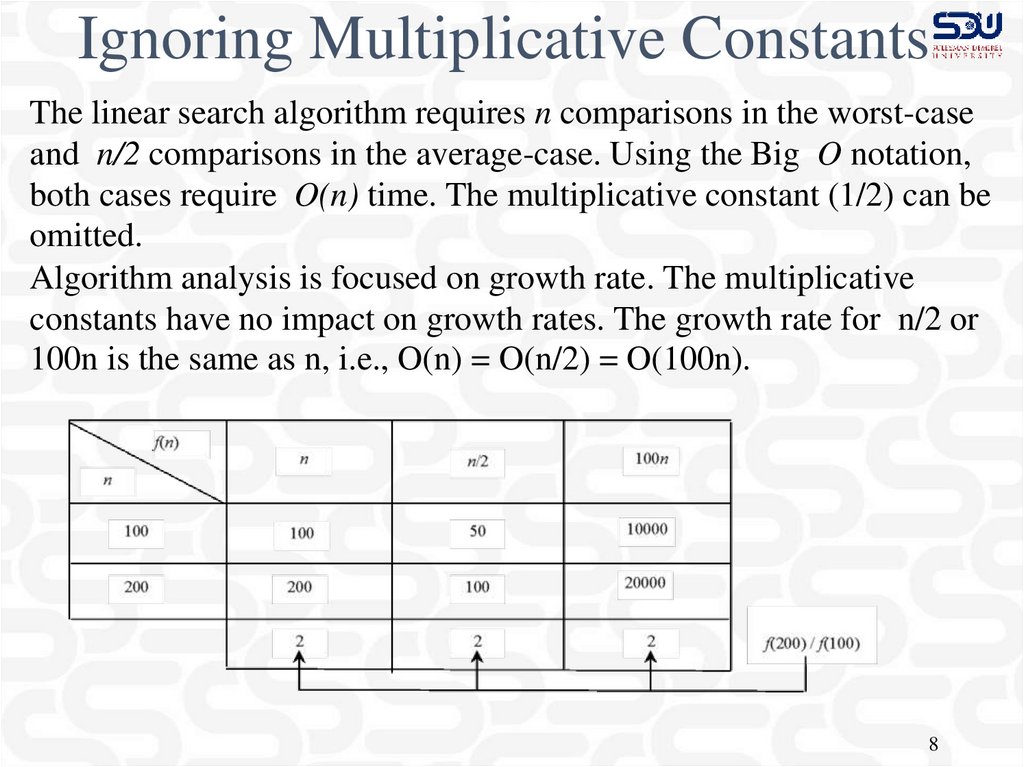
Ignoring Multiplicative ConstantsThe linear search algorithm requires n comparisons in the worst-case
and n/2 comparisons in the average-case. Using the Big O notation,
both cases require O(n) time. The multiplicative constant (1/2) can be
omitted.
Algorithm analysis is focused on growth rate. The multiplicative
constants have no impact on growth rates. The growth rate for n/2 or
100n is the same as n, i.e., O(n) = O(n/2) = O(100n).
8
9.
Ignoring Non-Dominating TermsConsider the algorithm for finding the maximum number in
an array of n elements. If n is 2, it takes one comparison to
find the maximum number. If n is 3, it takes two
comparisons to find the maximum number. In general, it
takes n-1 times of comparisons to find maximum number in
a list of n elements.
Algorithm analysis is for large input size. If the input size is
small, there is no significance to estimate an algorithm’s
efficiency. As n grows larger, the n part in the expression
n-1 dominates the complexity.
The Big O notation allows you to ignore the nondominating part (e.g., -1 in the expression n-1) and
highlight the important part (e.g., n in the expression n-1).
So, the complexity of this algorithm is O(n).
9
10.
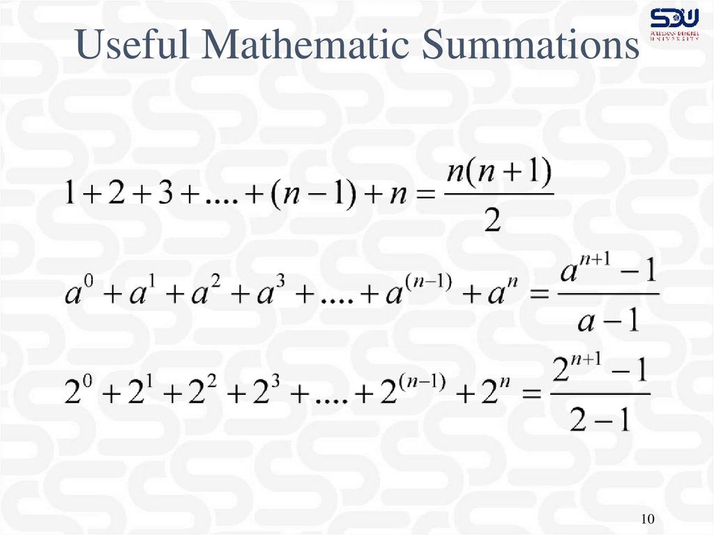
Useful Mathematic Summations10
11.
Examples: Determining Big-O▪
Repetition
▪
Sequence
▪
Selection
▪
Logarithm
11
12.
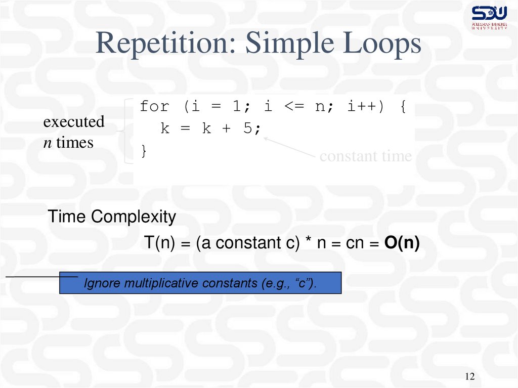
Repetition: Simple Loopsexecuted
n times
for (i = 1; i <= n; i++) {
k = k + 5;
}
constant time
Time Complexity
T(n) = (a constant c) * n = cn = O(n)
Ignore multiplicative constants (e.g., “c”).
12
13.
Repetition: Nested Loopsexecuted
n times
for (i = 1; i <= n; i++) {
for (j = 1; j <= n; j++) {
k = k + i + j;
}
}
constant time
inner loop
executed
n times
Time Complexity
T(n) = (a constant c) * n * n = cn2 = O(n2)
Ignore multiplicative constants (e.g., “c”).
13
14.
Repetition: Nested Loopsfor (i = 1; i <= n; i++) {
executed
for (j = 1; j <= i; j++) {
inner loop
n times
k = k + i + j;
executed
}
i times
}
constant time
Time Complexity
T(n) = c + 2c + 3c + 4c + … + nc = cn(n+1)/2 =
(c/2)n2 + (c/2)n = O(n2)
Ignore non-dominating terms
Ignore multiplicative constants
14
15.
Repetition: Nested Loopsexecuted
n times
for (i = 1; i <= n; i++) {
for (j = 1; j <= 20; j++) {
k = k + i + j;
}
}
constant time
inner loop
executed
20 times
Time Complexity
T(n) = 20 * c * n = O(n)
Ignore multiplicative constants (e.g., 20*c)
15
16.
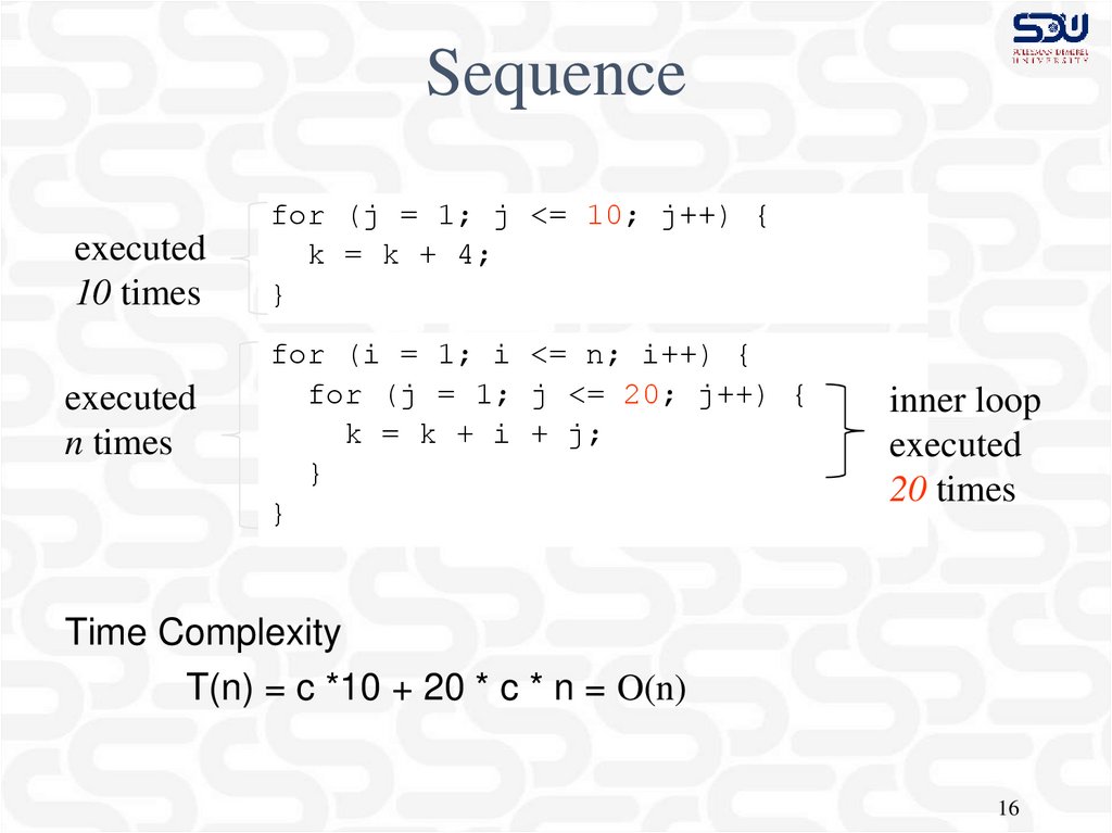
Sequenceexecuted
10 times
executed
n times
for (j = 1; j <= 10; j++) {
k = k + 4;
}
for (i = 1; i <= n; i++) {
for (j = 1; j <= 20; j++) {
k = k + i + j;
}
}
inner loop
executed
20 times
Time Complexity
T(n) = c *10 + 20 * c * n = O(n)
16
17.
O(n)Selection
if (list.contains(e)) {
System.out.println(e);
}
else
for (Object t: list) {
System.out.println(t);
}
Let n be
list.size().
Executed
n times.
Time Complexity
T(n) = test time + worst-case (if, else)
= O(n) + O(n)
= O(n)
17
18.
Constant TimeThe Big O notation estimates the execution time of an algorithm in
relation to the input size. If the time is not related to the input size, the
algorithm is said to take constant time with the notation O(1).
For example, a method that retrieves an element at a given index in an
array takes constant time, because it does not grow as the size of the
array increases.
18
19.
animationLinear Search Animation
http://www.cs.armstrong.edu/liang/animation/web/Linear
Search.html
19
20.
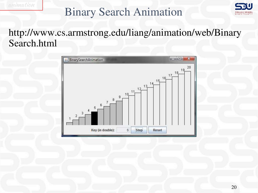
animationBinary Search Animation
http://www.cs.armstrong.edu/liang/animation/web/Binary
Search.html
20
21.
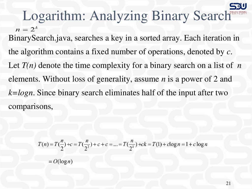
Logarithm: Analyzing Binary SearchBinarySearch.java, searches a key in a sorted array. Each iteration in
the algorithm contains a fixed number of operations, denoted by c.
Let T(n) denote the time complexity for a binary search on a list of n
elements. Without loss of generality, assume n is a power of 2 and
k=logn. Since binary search eliminates half of the input after two
comparisons,
21
22.
Logarithmic TimeIgnoring constants and smaller terms, the complexity of the
binary search algorithm is O(logn). An algorithm with the
O(logn) time complexity is called a logarithmic algorithm. The
base of the log is 2, but the base does not affect a logarithmic
growth rate, so it can be omitted. The logarithmic algorithm
grows slowly as the problem size increases. If you square the
input size, you only double the time for the algorithm.
22
23.
animationSelection Sort Animation
http://www.cs.armstrong.edu/liang/animation/web/Selecti
onSort.html
23
24.
Analyzing Selection SortSelection sort algorithm, SelectionSort.java, finds the smallest
number in the list and places it first. It then finds the smallest number
remaining and places it second, and so on until the list contains only a
single number. The number of comparisons is n-1 for the first
iteration, n-2 for the second iteration, and so on. Let T(n) denote the
complexity for selection sort and c denote the total number of other
operations such as assignments and additional comparisons in each
iteration. So,
Ignoring constants and smaller terms, the complexity of the selection
sort algorithm is O(n2).
24
25.
Quadratic TimeAn algorithm with the O(n2) time complexity is called a
quadratic algorithm. The quadratic algorithm grows
quickly as the problem size increases. If you double the
input size, the time for the algorithm is quadrupled.
Algorithms with a nested loop are often quadratic.
25
26.
Analyzing Selection SortIgnoring constants and smaller terms, the complexity of the selection
sort algorithm is O(n2).
26
27.
animationInsertion Sort Animation
http://www.cs.armstrong.edu/liang/animation/web/Insertio
nSort.html
27
28.
Analyzing Insertion SortThe insertion sort algorithm, InsertionSort.java, sorts a list of values
by repeatedly inserting a new element into a sorted partial array until
the whole array is sorted. At the kth iteration, to insert an element to a
array of size k, it may take k comparisons to find the insertion
position, and k moves to insert the element. Let T(n) denote the
complexity for insertion sort and c denote the total number of other
operations such as assignments and additional comparisons in each
iteration. So,
Ignoring constants and smaller terms, the complexity of the insertion
sort algorithm is O(n2).
28
29.
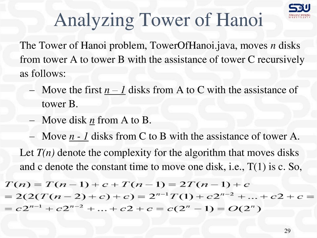
Analyzing Tower of HanoiThe Tower of Hanoi problem, TowerOfHanoi.java, moves n disks
from tower A to tower B with the assistance of tower C recursively
as follows:
– Move the first n – 1 disks from A to C with the assistance of
tower B.
– Move disk n from A to B.
– Move n - 1 disks from C to B with the assistance of tower A.
Let T(n) denote the complexity for the algorithm that moves disks
and c denote the constant time to move one disk, i.e., T(1) is c. So,
29
30.
Comparing Common Growth FunctionsConstant time
Logarithmic time
Linear time
Log-linear time
Quadratic time
Cubic time
Exponential time
30
31.
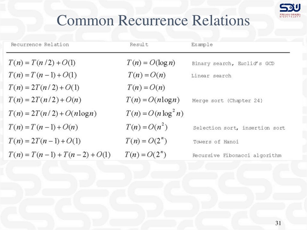
Common Recurrence Relations31
32.
Comparing Common Growth Functions32
33.
Case Study: Fibonacci Numbers/** The recursive method for finding the Fibonacci number */
public static long fib(long index) {
if (index == 0) // Base case
return 0;
else if (index == 1) // Base case
return 1;
else // Reduction and recursive calls
return fib(index - 1) + fib(index - 2);
}
Finonacci series: 0 1 1 2 3 5 8 13 21 34 55 89…
indices: 0 1 2 3 4 5 6 7
8
9
10 11
fib(0) = 0;
fib(1) = 1;
fib(index) = fib(index -1) + fib(index -2); index >=2
33
34.
Complexity for RecursiveFibonacci Numbers
Since
and
Therefore, the recursive Fibonacci method takes
34
35.
Case Study: Non-recursive versionof Fibonacci Numbers
public static long fib(long n) {
long f0 = 0; // For fib(0)
long f1 = 1; // For fib(1)
long f2 = 1; // For fib(2)
if (n == 0)
return f0;
else if (n == 1)
return f1;
else if (n == 2)
return f2;
Obviously, the complexity of
this new algorithm is
This is a tremendous
improvement over the
recursive algorithm.
for (int i = 3; i <= n; i++) {
f0 = f1;
f1 = f2;
f2 = f0 + f1;
}
return f2;
}
35
36.
f0 f1 f2Fibonacci series: 0 1 1 2 3 5 8 13 21 34 55 89…
indices: 0
1
2
3 4 5 6 7
8
9
10 11
f0 f1 f2
Fibonacci series: 0 1 1 2
3
5
8
13
21 34 55 89…
indices: 0
4
5
6
7
8
9
f0 f1 f2
1 1 2 3
5
8
13
21
34
55 89…
1
5
6
7
8
9
10 11
Fibonacci series: 0
indices: 0
1
2
2
3
3
4
10 11
Fibonacci series: 0
1
1
2
3
5
8
f0 f1 f2
13 21 34 55 89…
indices: 0
1
2
3
4
5
6
7
8
9
10 11
36
37.
Dynamic ProgrammingThe algorithm for computing Fibonacci numbers presented
here uses an approach known as dynamic programming.
Dynamic programming is to solve subproblems, then
combine the solutions of subproblems to obtain an overall
solution.
The key idea behind dynamic programming is to solve
each subprogram only once and storing the results for
subproblems for later use to avoid redundant (unnecessary)
computing of the subproblems.
37
38.
Case Study: Great CommonDivisor(GCD) Algorithms Version 1
public static int gcd(int m, int n) {
int gcd = 1;
for (int k = 2; k <= m && k <= n; k++) {
if (m % k == 0 && n % k == 0)
gcd = k;
}
return gcd;
}
Obviously, the complexity
of this algorithm is .
38
39.
Case Study: GCD AlgorithmsVersion 2
for (int k = n; k >= 1; k--) {
if (m % k == 0 && n % k == 0) {
gcd = k;
break;
}
}
The worst-case time complexity
of this algorithm is still .
39
40.
Case Study: GCD AlgorithmsVersion 3
public static int gcd(int m, int n) {
int gcd = 1;
if (m == n) return m;
for (int k = n / 2; k >= 1; k--) {
if (m % k == 0 && n % k == 0) {
gcd = k;
break;
}
}
return gcd;
}
The worst-case time complexity
of this algorithm is still .
40
41.
Euclid’s algorithmLet gcd(m, n) denote (indicate) the gcd for
integers m and n:
If m % n is 0, gcd (m, n) is n.
For example: gcd(12,6)=6
Otherwise, gcd(m, n) is gcd(n, m % n).
m = n*k + r
if p is divisible by both m and n,
it must be divisible by r
m / p = n*k/p + r/p
41
42.
Euclid’s Algorithm Implementationpublic static int gcd(int m, int n) {
if (m % n == 0)
return n;
else
return gcd(n, m % n);
}
The time complexity of this
algorithm is O(logn).
42
43.
Finding Prime NumbersCompare three versions:
▪
▪
▪
PrimeNumbers
Brute-force PrimeNumber
Check possible divisors up to Math.sqrt(n)
Check possible prime divisors up to
Math.sqrt(n)
EfficientPrimeNumbers
SieveOfEratosthenes
43
44.
Comparisons of Prime-Number Algorithms44
45.
Divide-and-ConquerThe divide-and-conquer approach divides the
problem into subproblems, solves the subproblems,
then combines the solutions of subproblems to
obtain the solution for the entire problem.
Unlike the dynamic programming approach, the
subproblems in the divide-and-conquer approach
don’t overlap.
A subproblem is like the original problem with a
smaller size, so you can apply recursion to solve
the problem. In fact, all the recursive problems
follow the divide-and-conquer approach.
45
46.
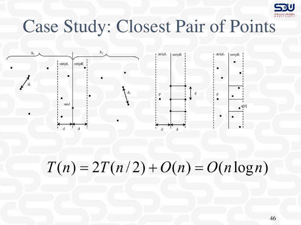
Case Study: Closest Pair of Points46
47.
Case Study: Closest Pair of Points47
48.
Eight QueensEightQueens
48
49.
animationBacktracking
There are many possible candidates? How do you
find a solution? The backtracking approach is to
search for a candidate incrementally and abandons
it as soon as it determines that the candidate cannot
possibly be a valid solution, and explores a new
candidate.
http://www.cs.armstrong.edu/liang/animation/EightQueensAnimation.html
49
50.
Eight Queens50
51.
animationConvex Hull Animation
http://www.cs.armstrong.edu/liang/animation/web/Conve
xHull.html
51
52.
Convex HullGiven a set of points, a convex hull is a smallest convex
polygon that encloses all these points, as shown in Figure a.
A polygon is convex if every line connecting two vertices
is inside the polygon. For example, the vertices v0, v1, v2,
v3, v4, and v5 in Figure a form a convex polygon, but not
in Figure b, because the line that connects v3 and v1 is not
inside the polygon.
Figure a
Figure b
52
53.
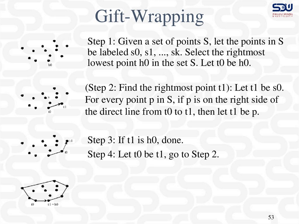
Gift-WrappingStep 1: Given a set of points S, let the points in S
be labeled s0, s1, ..., sk. Select the rightmost
lowest point h0 in the set S. Let t0 be h0.
(Step 2: Find the rightmost point t1): Let t1 be s0.
For every point p in S, if p is on the right side of
the direct line from t0 to t1, then let t1 be p.
Step 3: If t1 is h0, done.
Step 4: Let t0 be t1, go to Step 2.
53
54.
Gift-Wrapping Algorithm TimeFinding the rightmost lowest point in Step 1
can be done in O(n) time.
Whether a point is on the left side of a line,
right side, or on the line can decided in O(1)
time.
Thus, it takes O(n) time to find a new point t1
in Step 2. Step 2 is repeated h times, where h
is the size of the convex hull.
Therefore, the algorithm takes O(hn) time. In
the worst case, h is n.
54
55.
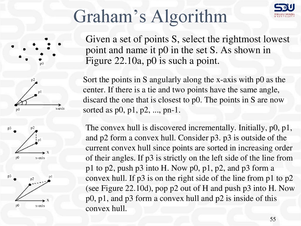
Graham’s AlgorithmGiven a set of points S, select the rightmost lowest
point and name it p0 in the set S. As shown in
Figure 22.10a, p0 is such a point.
Sort the points in S angularly along the x-axis with p0 as the
center. If there is a tie and two points have the same angle,
discard the one that is closest to p0. The points in S are now
sorted as p0, p1, p2, ..., pn-1.
The convex hull is discovered incrementally. Initially, p0, p1,
and p2 form a convex hull. Consider p3. p3 is outside of the
current convex hull since points are sorted in increasing order
of their angles. If p3 is strictly on the left side of the line from
p1 to p2, push p3 into H. Now p0, p1, p2, and p3 form a
convex hull. If p3 is on the right side of the line from p1 to p2
(see Figure 22.10d), pop p2 out of H and push p3 into H. Now
p0, p1, and p3 form a convex hull and p2 is inside of this
convex hull.
55
56.
Graham’s Algorithm TimeO(nlogn)
56
57.
Practical ConsiderationsThe big O notation provides a good theoretical
estimate of algorithm efficiency. However, two
algorithms of the same time complexity are not
necessarily equally efficient. As shown in the
preceding example, both algorithms in Listings 4.6
and 22.2 have the same complexity, but the one in
Listing 22.2 is obviously better practically.
57