


 Программирование
Похожие презентации:

. Τάξεις και αφαίρεση δεδομένων")


 and the fundamental tree algorithm")

")
")
Assignment Method
1.
Assignment Method© 2006
Prentice
Hall, Inc. Hall, Inc.
©
2006
Prentice
15 – 1
2.
What is the Assignment Method?The assignment method is any technique used to
assign organizational resources to activities. The
best assignment method will maximize profits,
typically
through
cost
controls,
increases
in
efficiency
levels,
and
better
management
of
bottleneck operations.
© 2006 Prentice Hall, Inc.
15 – 2
3.
Assignment MethodA special class of linear
programming models that assign
tasks or jobs( programming,
analyzing, Design..) to resources
Objective is to minimize cost or
time
Only one job (or programmer) is
assigned to one computer (or
project)
© 2006 Prentice Hall, Inc.
15 – 3
4.
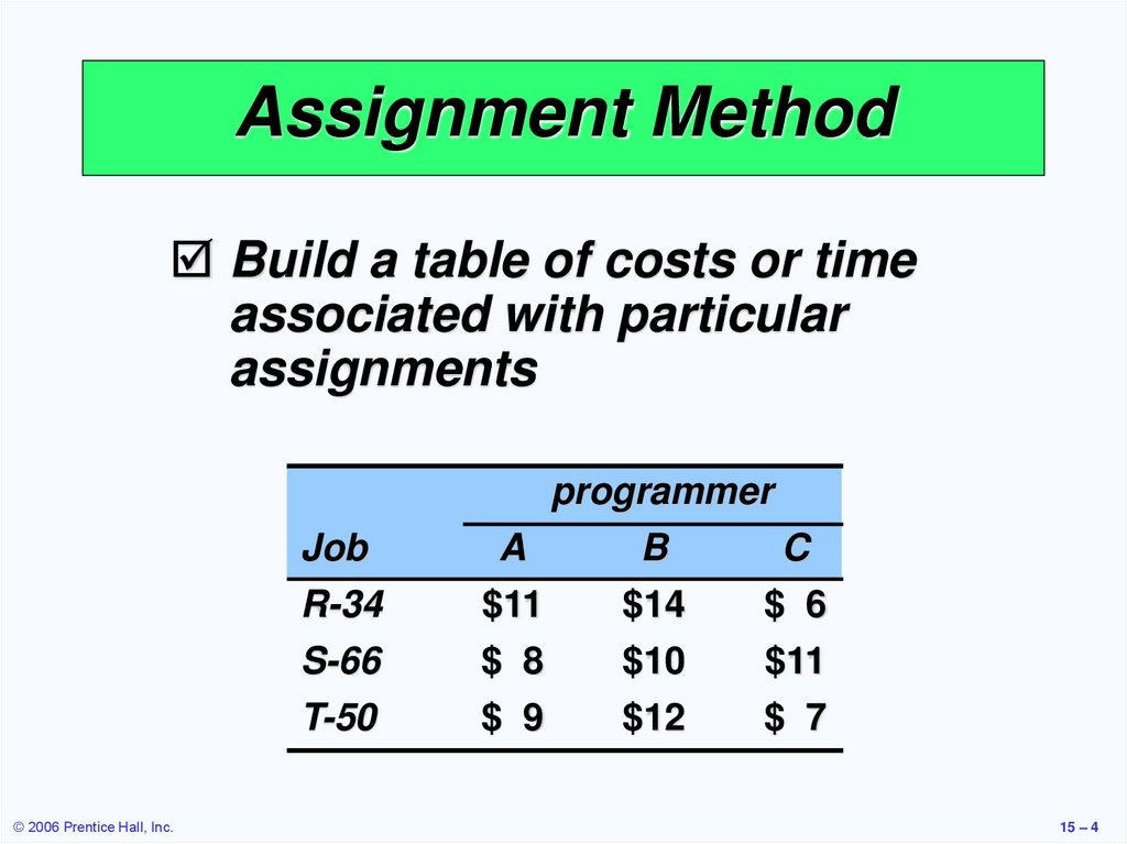
Assignment MethodBuild a table of costs or time
associated with particular
assignments
Job
R-34
S-66
T-50
© 2006 Prentice Hall, Inc.
programmer
A
B
C
$11
$14
$ 6
$ 8
$10
$11
$ 9
$12
$ 7
15 – 4
5.
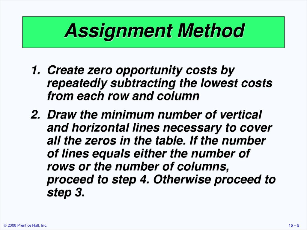
Assignment Method1. Create zero opportunity costs by
repeatedly subtracting the lowest costs
from each row and column
2. Draw the minimum number of vertical
and horizontal lines necessary to cover
all the zeros in the table. If the number
of lines equals either the number of
rows or the number of columns,
proceed to step 4. Otherwise proceed to
step 3.
© 2006 Prentice Hall, Inc.
15 – 5
6.
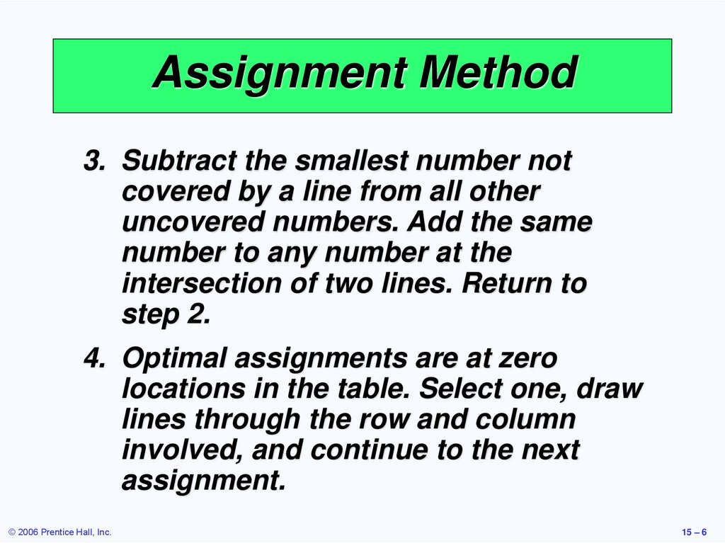
Assignment Method3. Subtract the smallest number not
covered by a line from all other
uncovered numbers. Add the same
number to any number at the
intersection of two lines. Return to
step 2.
4. Optimal assignments are at zero
locations in the table. Select one, draw
lines through the row and column
involved, and continue to the next
assignment.
© 2006 Prentice Hall, Inc.
15 – 6
7.
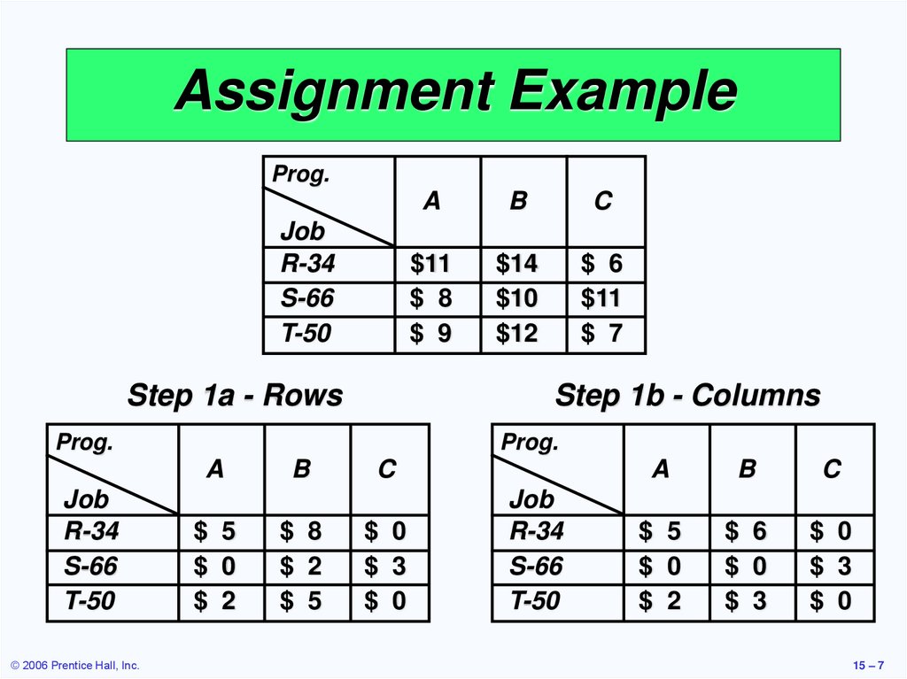
Assignment ExampleProg.
Job
R-34
S-66
T-50
Step 1a - Rows
C
$11
$ 8
$ 9
$14
$10
$12
$ 6
$11
$ 7
Prog.
A
© 2006 Prentice Hall, Inc.
B
Step 1b - Columns
Prog.
Job
R-34
S-66
T-50
A
$ 5
$ 0
$ 2
B
$ 8
$ 2
$ 5
C
$ 0
$ 3
$ 0
Job
R-34
S-66
T-50
A
B
C
$ 5
$ 0
$ 2
$ 6
$ 0
$ 3
$ 0
$ 3
$ 0
15 – 7
8.
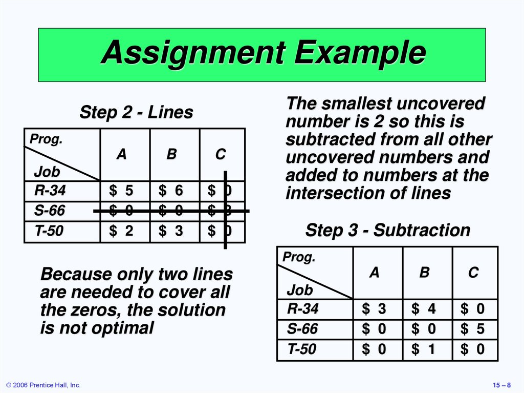
Assignment ExampleStep 2 - Lines
Prog.
Job
R-34
S-66
T-50
A
B
C
$ 5
$ 0
$ 2
$ 6
$ 0
$ 3
$ 0
$ 3
$ 0
The smallest uncovered
number is 2 so this is
subtracted from all other
uncovered numbers and
added to numbers at the
intersection of lines
Step 3 - Subtraction
Prog.
Because only two lines
are needed to cover all
the zeros, the solution
is not optimal
© 2006 Prentice Hall, Inc.
Job
R-34
S-66
T-50
A
B
C
$ 3
$ 0
$ 0
$ 4
$ 0
$ 1
$ 0
$ 5
$ 0
15 – 8
9.
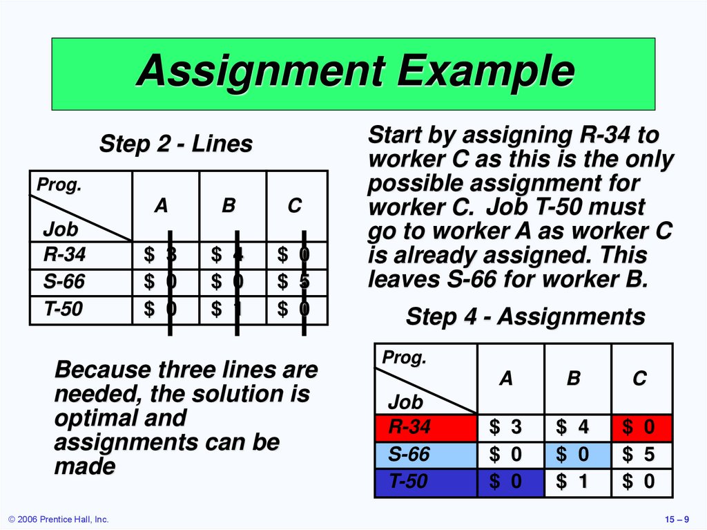
Assignment ExampleStep 2 - Lines
Prog.
Job
R-34
S-66
T-50
A
B
C
$ 3
$ 0
$ 0
$ 4
$ 0
$ 1
$ 0
$ 5
$ 0
Because three lines are
needed, the solution is
optimal and
assignments can be
made
© 2006 Prentice Hall, Inc.
Start by assigning R-34 to
worker C as this is the only
possible assignment for
worker C. Job T-50 must
go to worker A as worker C
is already assigned. This
leaves S-66 for worker B.
Step 4 - Assignments
Prog.
Job
R-34
S-66
T-50
A
B
C
$ 3
$ 0
$ 0
$ 4
$ 0
$ 1
$ 0
$ 5
$ 0
15 – 9
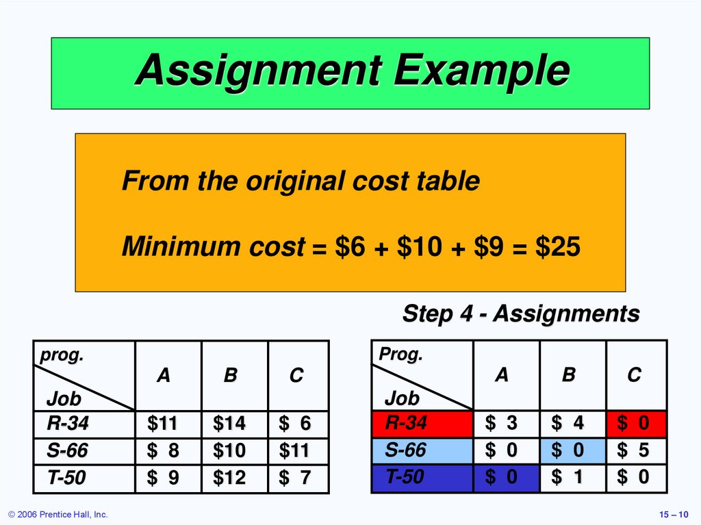
10.
Assignment ExampleFrom the original cost table
Minimum cost = $6 + $10 + $9 = $25
Step 4 - Assignments
Prog.
prog.
A
Job
R-34
S-66
T-50
© 2006 Prentice Hall, Inc.
$11
$ 8
$ 9
B
$14
$10
$12
C
$ 6
$11
$ 7
Job
R-34
S-66
T-50
A
B
C
$ 3
$ 0
$ 0
$ 4
$ 0
$ 1
$ 0
$ 5
$ 0
15 – 10
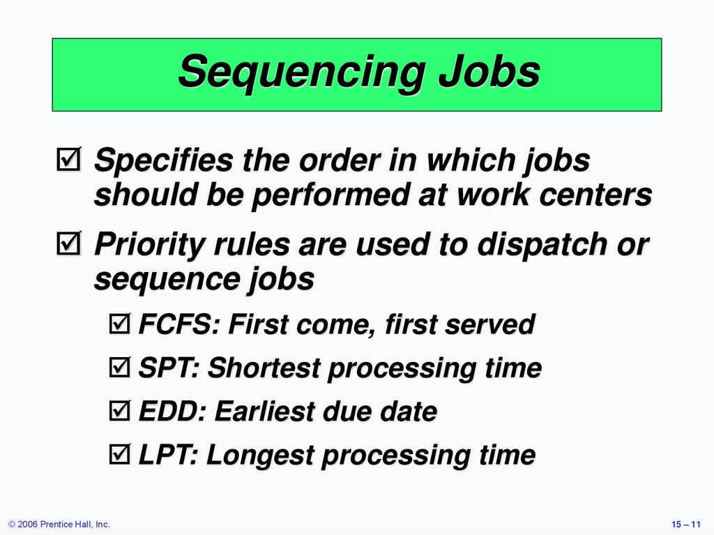
11.
Sequencing JobsSpecifies the order in which jobs
should be performed at work centers
Priority rules are used to dispatch or
sequence jobs
FCFS: First come, first served
SPT: Shortest processing time
EDD: Earliest due date
LPT: Longest processing time
© 2006 Prentice Hall, Inc.
15 – 11
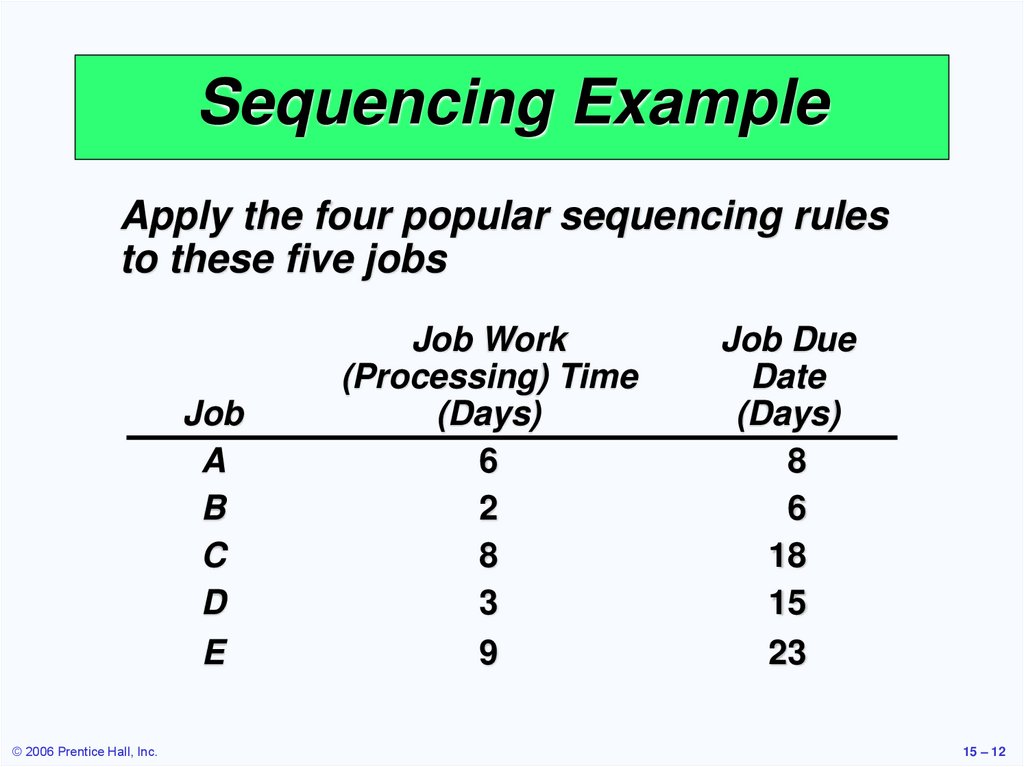
12.
Sequencing ExampleApply the four popular sequencing rules
to these five jobs
Job
A
B
C
D
E
© 2006 Prentice Hall, Inc.
Job Work
(Processing) Time
(Days)
6
2
8
3
9
Job Due
Date
(Days)
8
6
18
15
23
15 – 12
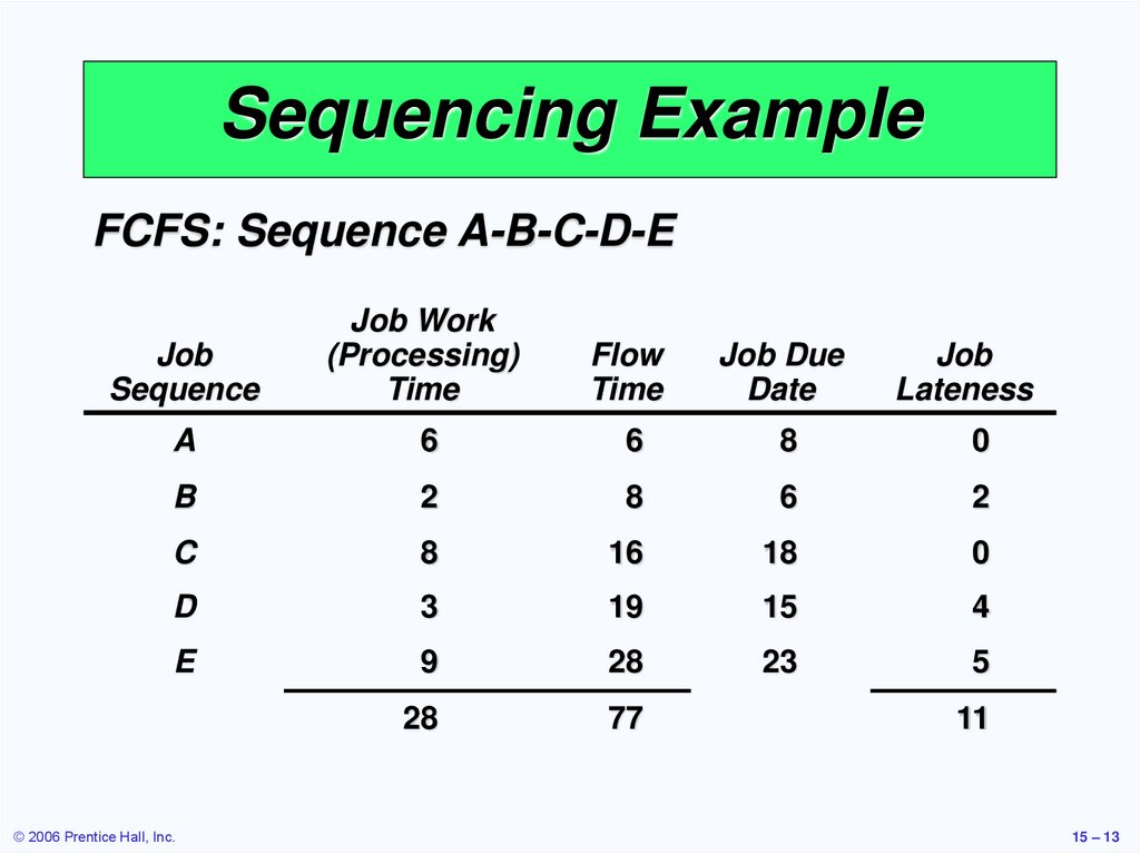
13.
Sequencing ExampleFCFS: Sequence A-B-C-D-E
Job
Sequence
Job Work
(Processing)
Time
Flow
Time
Job Due
Date
Job
Lateness
A
6
6
8
0
B
2
8
6
2
C
8
16
18
0
D
3
19
15
4
E
9
28
23
5
28
77
© 2006 Prentice Hall, Inc.
11
15 – 13
14.
Sequencing ExampleFCFS: Sequence A-B-C-D-E
Total flow time
Jobtime
Work
Average completion
=
= 77/5 = 15.4 days
Job
(Processing) Number
Flowof jobs
Job Due
Job
Sequence
Time
Time
Date
Lateness
Total job work time
= 28/77
A Utilization = 6Total flow time
6
8 = 36.4% 0
B
2
8
6
2
Total flow time
Average number of
= 77/28 = 2.75 jobs
jobsCin the system =8 Total job work
16 time 18
0
D
3
19 days 15
4
Total late
Average job lateness = Number of jobs = 11/5 = 2.2 days
E
9
28
23
5
28
© 2006 Prentice Hall, Inc.
77
11
15 – 14
15.
Sequencing ExampleSPT: Sequence B-D-A-C-E
Job
Sequence
Job Work
(Processing)
Time
Flow
Time
Job Due
Date
Job
Lateness
B
2
2
6
0
D
3
5
15
0
A
6
11
8
3
C
8
19
18
1
E
9
28
23
5
28
65
© 2006 Prentice Hall, Inc.
9
15 – 15
16.
Sequencing ExampleSPT: Sequence B-D-A-C-E
Total flow time
Job Work
Average completion
time =
= 65/5 = 13 days
Job
(Processing) Number
Flow of jobs
Job Due
Job
Sequence
Time
Time
Date
Lateness
Total job work time
= 28/65
B Utilization = 2Total flow time
2
6 = 43.1% 0
D
3
5
15
0
Total flow time
Average number of
= 65/28 = 2.32 jobs
jobsAin the system =6 Total job work
11 time 8
3
C
8
19 days 18
1
Total late
Average job lateness = Number of jobs = 9/5 = 1.8 days
E
9
28
23
5
28
© 2006 Prentice Hall, Inc.
65
9
15 – 16
17.
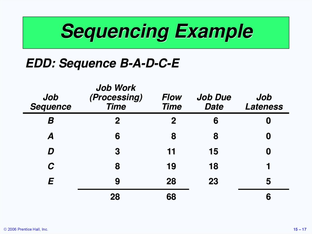
Sequencing ExampleEDD: Sequence B-A-D-C-E
Job
Sequence
Job Work
(Processing)
Time
Flow
Time
Job Due
Date
Job
Lateness
B
2
2
6
0
A
6
8
8
0
D
3
11
15
0
C
8
19
18
1
E
9
28
23
5
28
68
© 2006 Prentice Hall, Inc.
6
15 – 17
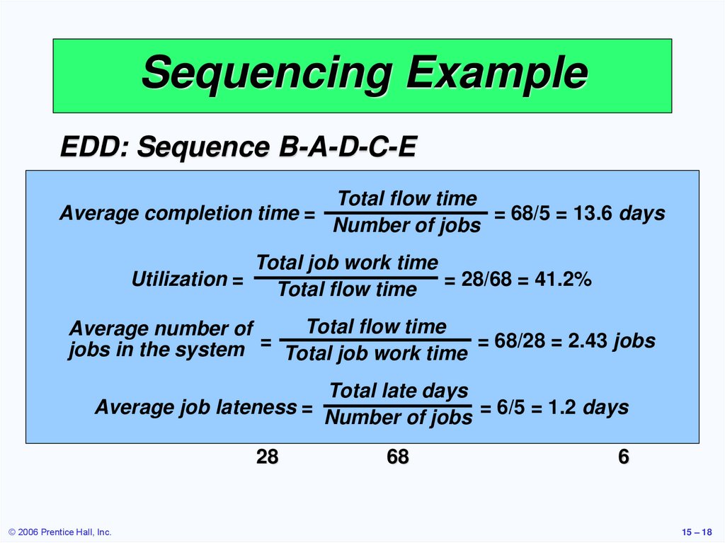
18.
Sequencing ExampleEDD: Sequence B-A-D-C-E
Total flow time
Jobtime
Work
Average completion
=
= 68/5 = 13.6 days
Job
(Processing) Number
Flowof jobs
Job Due
Job
Sequence
Time
Time
Date
Lateness
Total job work time
= 28/68
B Utilization = 2Total flow time
2
6 = 41.2% 0
A
6
8
8
0
Total flow time
Average number of
= 68/28 = 2.43 jobs
jobsDin the system =3 Total job work
11 time 15
0
C
8
19 days 18
1
Total late
Average job lateness = Number of jobs = 6/5 = 1.2 days
E
9
28
23
5
28
© 2006 Prentice Hall, Inc.
68
6
15 – 18
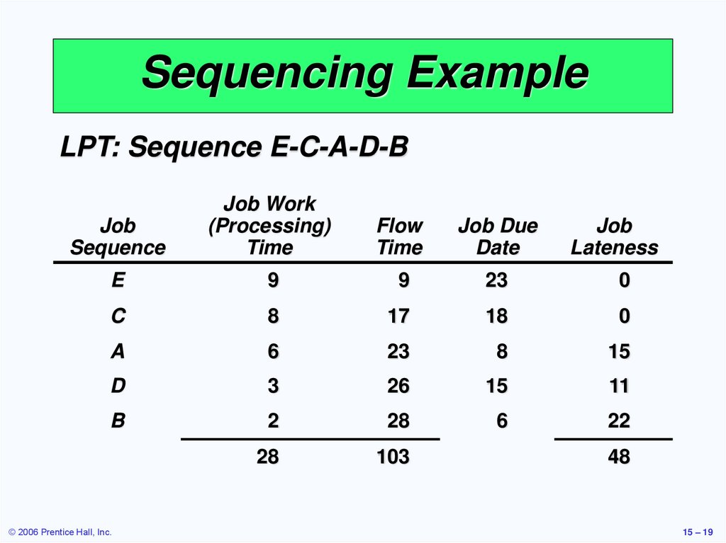
19.
Sequencing ExampleLPT: Sequence E-C-A-D-B
Job
Sequence
Job Work
(Processing)
Time
Flow
Time
Job Due
Date
Job
Lateness
E
9
9
23
0
C
8
17
18
0
A
6
23
8
15
D
3
26
15
11
B
2
28
6
22
28
103
© 2006 Prentice Hall, Inc.
48
15 – 19
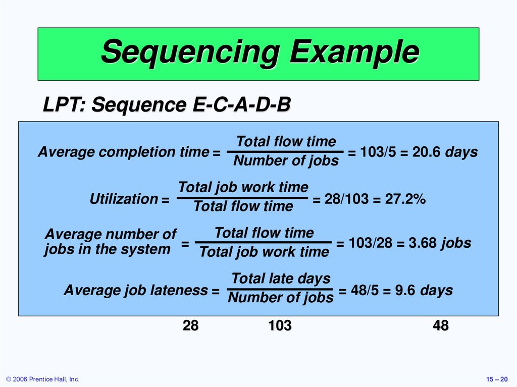
20.
Sequencing ExampleLPT: Sequence E-C-A-D-B
Total flow time
Jobtime
Work
Average completion
=
= 103/5 = 20.6 days
of jobs
Job
(Processing)Number
Flow
Job Due
Job
Sequence
Time
Time
Date
Lateness
Total job work time
EUtilization = 9Total flow time
9 = 28/103
23 = 27.2% 0
C
8
17
18
0
Total flow time
Average number of
=
= 103/28 = 3.68 jobs
jobs in
A the system 6Total job work
23 time
8
15
D
3
26 days 15
11
Total late
Average job lateness = Number of jobs = 48/5 = 9.6 days
B
2
28
6
22
28
© 2006 Prentice Hall, Inc.
103
48
15 – 20
21.
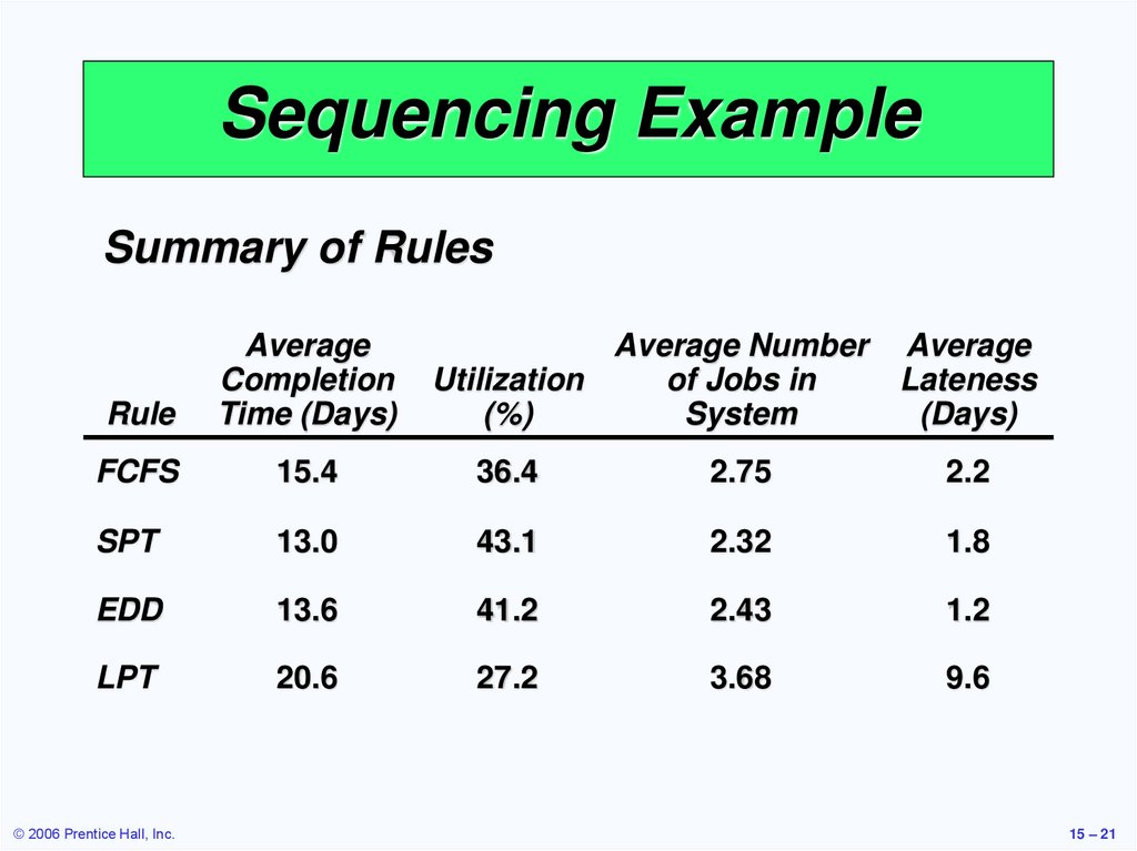
Sequencing ExampleSummary of Rules
Rule
Average
Completion
Time (Days)
FCFS
15.4
36.4
2.75
2.2
SPT
13.0
43.1
2.32
1.8
EDD
13.6
41.2
2.43
1.2
LPT
20.6
27.2
3.68
9.6
© 2006 Prentice Hall, Inc.
Average Number Average
Utilization
of Jobs in
Lateness
(%)
System
(Days)
15 – 21
22.
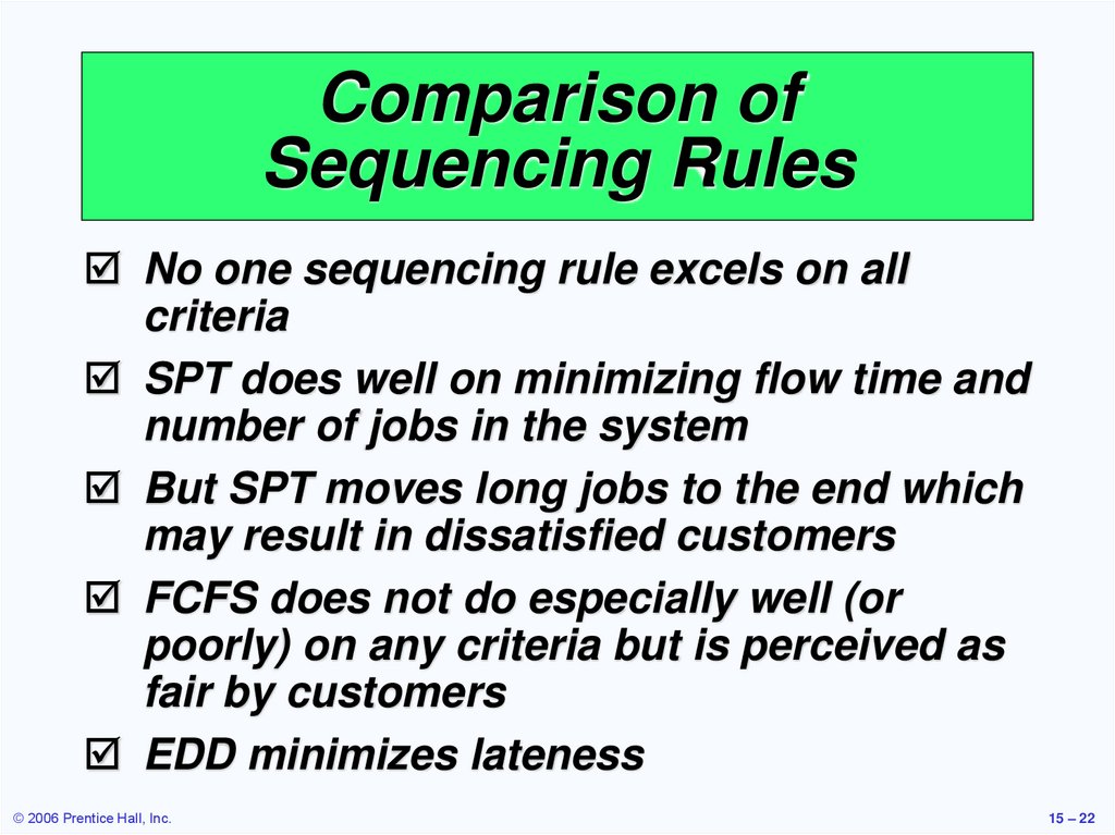
Comparison ofSequencing Rules
No one sequencing rule excels on all
criteria
SPT does well on minimizing flow time and
number of jobs in the system
But SPT moves long jobs to the end which
may result in dissatisfied customers
FCFS does not do especially well (or
poorly) on any criteria but is perceived as
fair by customers
EDD minimizes lateness
© 2006 Prentice Hall, Inc.
15 – 22
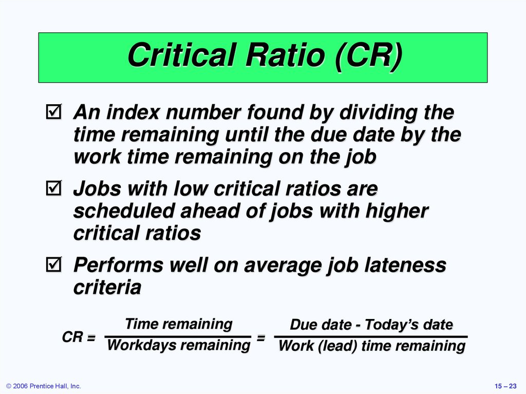
23.
Critical Ratio (CR)An index number found by dividing the
time remaining until the due date by the
work time remaining on the job
Jobs with low critical ratios are
scheduled ahead of jobs with higher
critical ratios
Performs well on average job lateness
criteria
Time remaining
Due date - Today’s date
CR =
=
Workdays remaining
Work (lead) time remaining
© 2006 Prentice Hall, Inc.
15 – 23
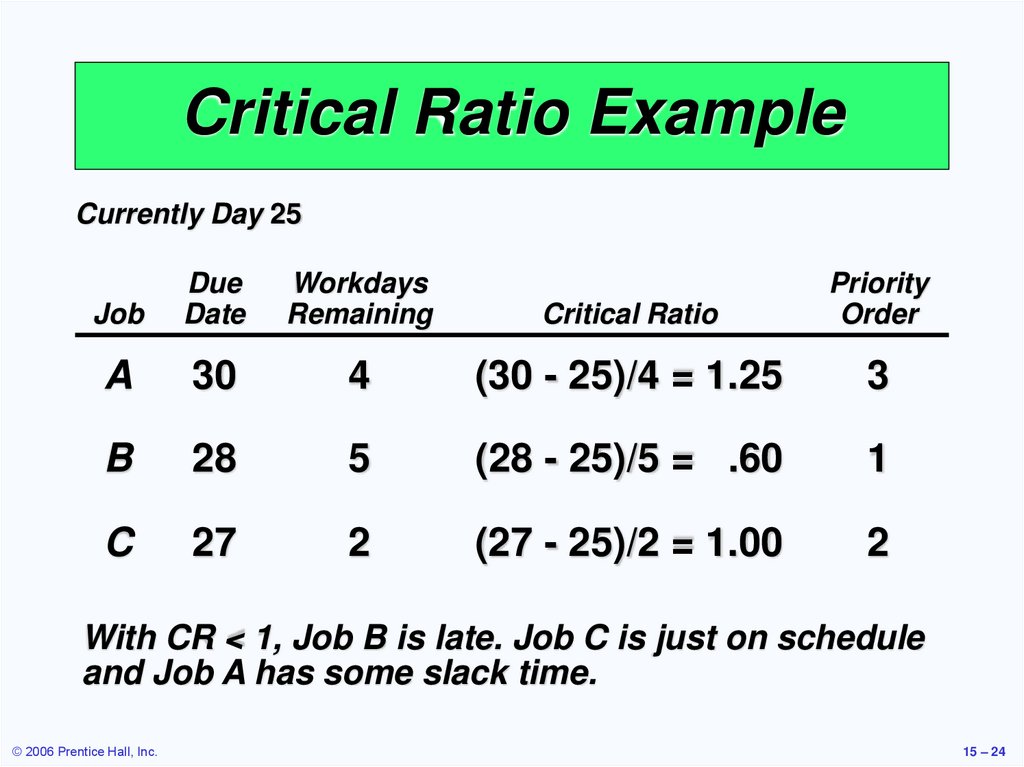
24.
Critical Ratio ExampleCurrently Day 25
Job
Due
Date
Workdays
Remaining
Critical Ratio
Priority
Order
A
30
4
(30 - 25)/4 = 1.25
3
B
28
5
(28 - 25)/5 = .60
1
C
27
2
(27 - 25)/2 = 1.00
2
With CR < 1, Job B is late. Job C is just on schedule
and Job A has some slack time.
© 2006 Prentice Hall, Inc.
15 – 24
25.
Critical Ratio Technique1. Helps determine the status of specific
jobs
2. Establishes relative priorities among
jobs on a common basis
3. Relates both stock and make-to-order
jobs on a common basis
4. Adjusts priorities automatically for
changes in both demand and job
progress
5. Dynamically tracks job progress
© 2006 Prentice Hall, Inc.
15 – 25
26.
Limitations of Rule-BasedDispatching Systems
1. Scheduling is dynamic and rules
need to be revised to adjust to
changes
2. Rules do not look upstream or
downstream
3. Rules do not look beyond due
dates
© 2006 Prentice Hall, Inc.
15 – 26
27.
Finite Capacity SchedulingOvercomes disadvantages of rule-based
systems by providing an interactive,
computer-based graphical system
May include rules and expert systems or
simulation to allow real-time response to
system changes
Initial data often from an MRP system
FCS allows the balancing of delivery
needs and efficiency
© 2006 Prentice Hall, Inc.
15 – 27
28.
Theory of ConstraintsThroughput is the number of units
processed through the facility and sold
TOC deals with the limits an organization
faces in achieving its goals
1. Identify the constraints
2. Develop a plan for overcoming the constraints
3. Focus resources on accomplishing the plan
4. Reduce the effects of constraints by offloading work or increasing capacity
5. Once successful, return to step 1 and identify
new constraints
© 2006 Prentice Hall, Inc.
15 – 28
29.
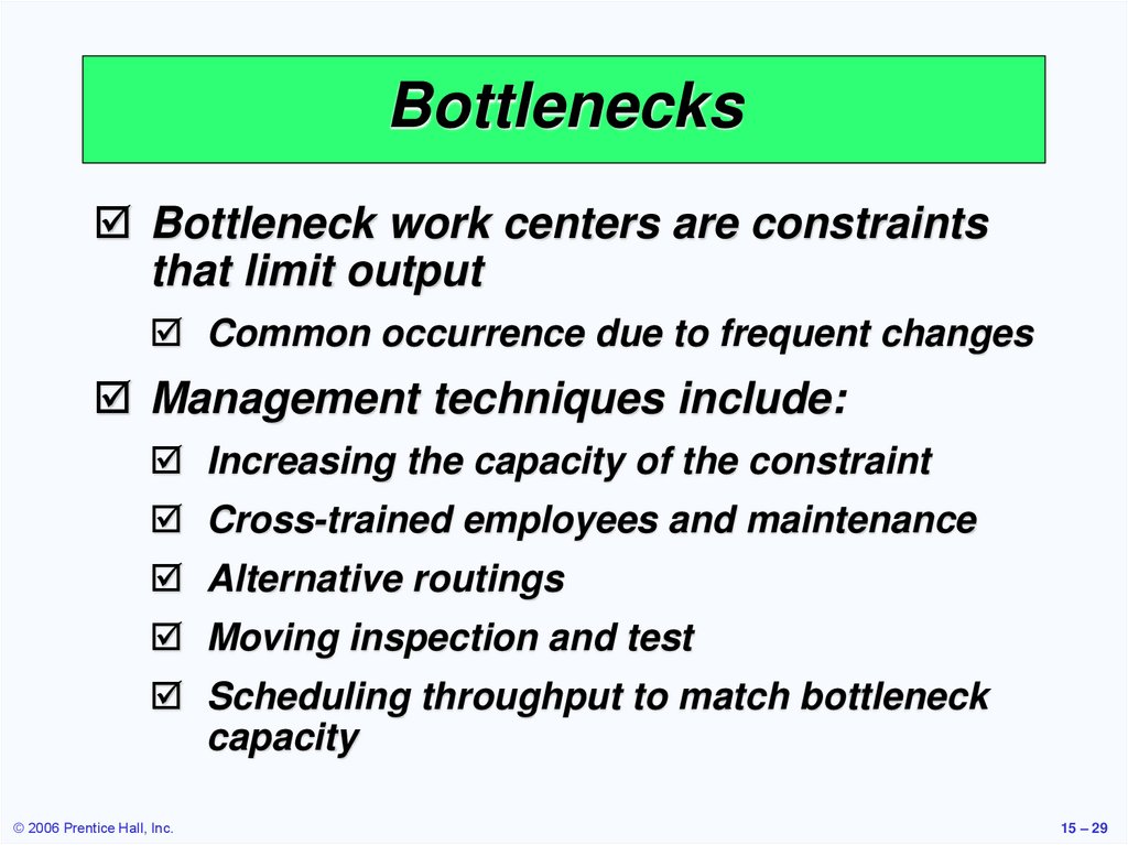
BottlenecksBottleneck work centers are constraints
that limit output
Common occurrence due to frequent changes
Management techniques include:
Increasing the capacity of the constraint
Cross-trained employees and maintenance
Alternative routings
Moving inspection and test
Scheduling throughput to match bottleneck
capacity
© 2006 Prentice Hall, Inc.
15 – 29
30.
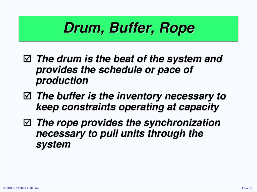
Drum, Buffer, RopeThe drum is the beat of the system and
provides the schedule or pace of
production
The buffer is the inventory necessary to
keep constraints operating at capacity
The rope provides the synchronization
necessary to pull units through the
system
© 2006 Prentice Hall, Inc.
15 – 30
31.
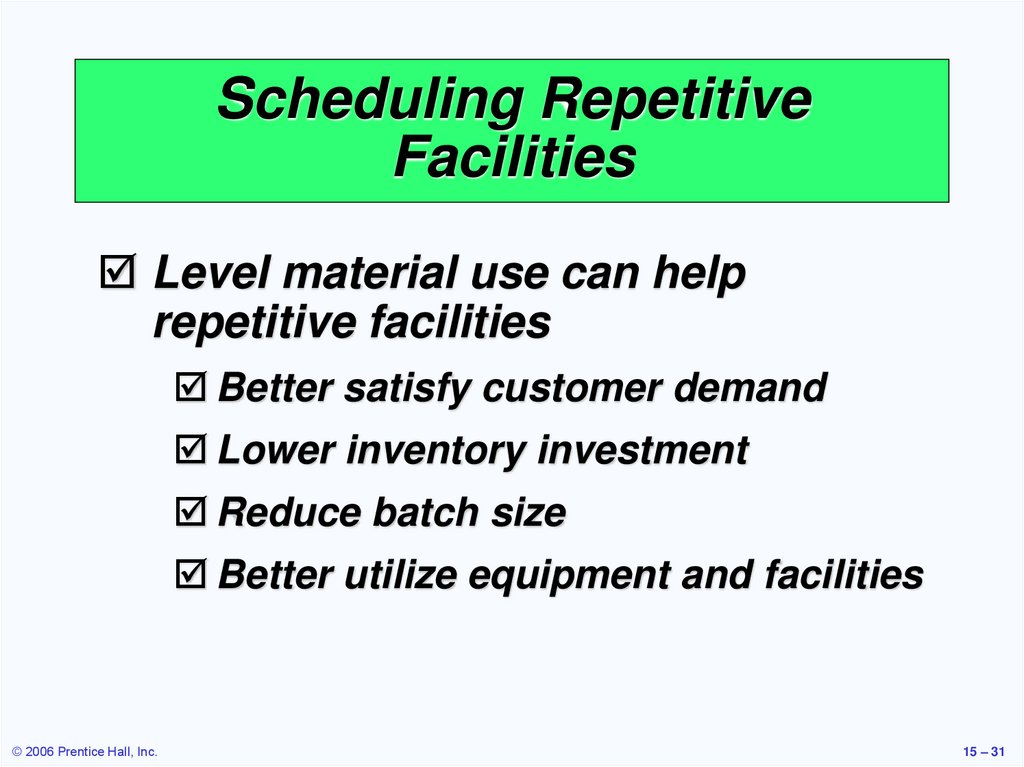
Scheduling RepetitiveFacilities
Level material use can help
repetitive facilities
Better satisfy customer demand
Lower inventory investment
Reduce batch size
Better utilize equipment and facilities
© 2006 Prentice Hall, Inc.
15 – 31
32.
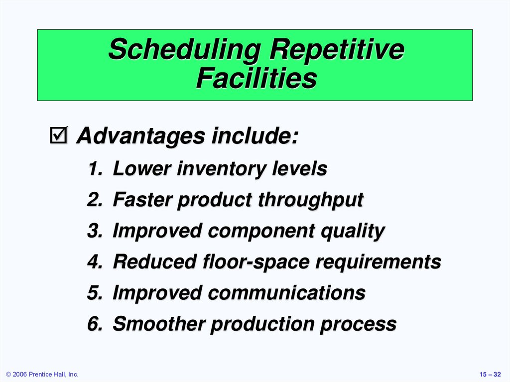
Scheduling RepetitiveFacilities
Advantages include:
1. Lower inventory levels
2. Faster product throughput
3. Improved component quality
4. Reduced floor-space requirements
5. Improved communications
6. Smoother production process
© 2006 Prentice Hall, Inc.
15 – 32
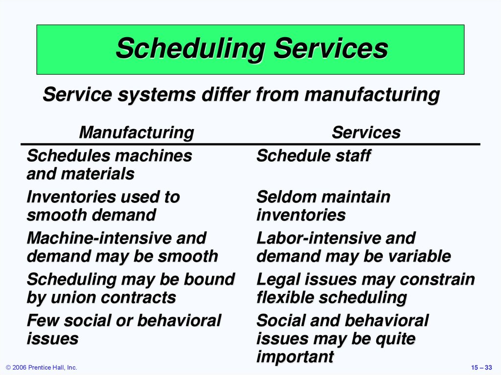
33.
Scheduling ServicesService systems differ from manufacturing
Manufacturing
Schedules machines
and materials
Inventories used to
smooth demand
Machine-intensive and
demand may be smooth
Scheduling may be bound
by union contracts
Few social or behavioral
issues
© 2006 Prentice Hall, Inc.
Services
Schedule staff
Seldom maintain
inventories
Labor-intensive and
demand may be variable
Legal issues may constrain
flexible scheduling
Social and behavioral
issues may be quite
important
15 – 33
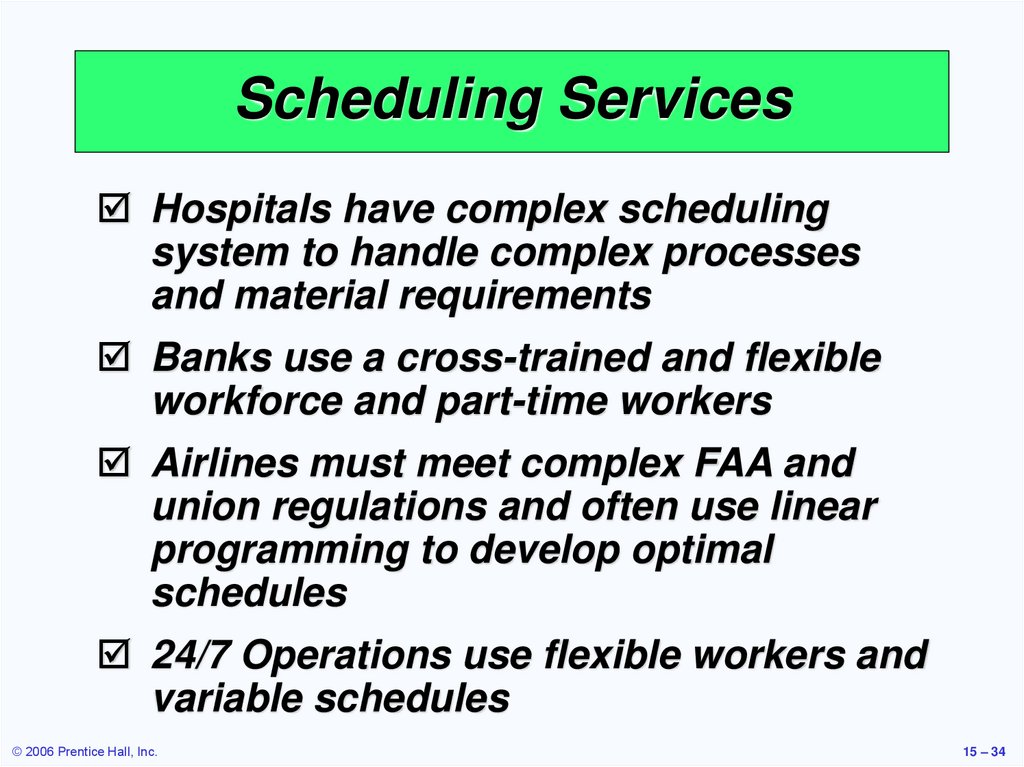
34.
Scheduling ServicesHospitals have complex scheduling
system to handle complex processes
and material requirements
Banks use a cross-trained and flexible
workforce and part-time workers
Airlines must meet complex FAA and
union regulations and often use linear
programming to develop optimal
schedules
24/7 Operations use flexible workers and
variable schedules
© 2006 Prentice Hall, Inc.
15 – 34
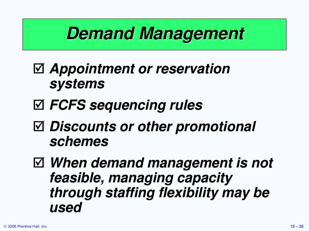
35.
Demand ManagementAppointment or reservation
systems
FCFS sequencing rules
Discounts or other promotional
schemes
When demand management is not
feasible, managing capacity
through staffing flexibility may be
used
© 2006 Prentice Hall, Inc.
15 – 35