Solving ultimate pit limit problem through graph closure (L-G algorithm) and the fundamental tree algorithm

1. SOLVING ULTIMATE PIT LIMIT PROBLEM THROUGH GRAPH CLOSURE (L-G ALGORITHM) AND THE FUNDAMENTAL TREE ALGORITHM

2. Contents

1. Introduction
2. Lerchs – Grossmann (Graph closure)
3. Fundamental Tree Algorithm
4. Assignment

3. Introduction

1. Introduction
Two ojectives for open pit optimization
Design ultimate pit limits (Moving cone, LG, Net work
flows …. )
Determining an optimal sequence of extracting the
mineralized material from the ground (Short-term and
Long-term production scheduling).
1.
Lerchs, H., and Grossmann, I. F., 1965. Optimum Design of
Open Pit Mines, Canad. Inst. Mining Bull. 58, pp. 47-54.
2.
Salih Ramazan, The new Fundamental Tree Algorithm for
production scheduling of open pit mines, European Journal of
Operational Research 177 (2007) 1153–1166

4. Block model

• gdg
Source:
William Hustrulid: Open Pit Mine Planning & Design

5.

DEPOSIT REPRESENTATION OREBODY MODEL
A set of mining blocks of a given size with block value
(Grade Recovery Price costp) OreTons
Waste Ore Tons costm, if grade > a cutoff grade
BV
Tons Waste costm, Otherwise
BV: Economic Value of a mining block

6.

DEPOSIT REPRESENTATION OREBODY MODEL
Geologic Model, Copper Grades (lb/ton)
Economic Model, Value per block ($/ton)

7. Ultimate Pit Limit Problems

Moving (Floating) Cone Algorithm
Dynamic Programming (LG)
Graph closure (Lerchs-Grossmann,
Minimum Cut , Pseudo-flow Algorithm)

8. 2. Graph closure (LG)

• The optimal pit outline is the 3D pit outline
which, if mined out, would give the maximum
value
– Must obey the required pit slope constraints
• All the ore which at a given time can be mined at
a profit will be mined
• Nothing can be added to or taken away from the
optimal outline which will increase the value
without breaking the slope constraints

9. Lerchs-Grossman Algorithm

Mathematical search technique which works from
just two sources of information:
1. Economic or value block model:
Set of regular rectangular blocks which completely fill
the space under consideration for mining
2. A list of relationships between these blocks:
These relationships are known as `arcs'

10. Arc Relationships

B
Arc
from
A to B
A
Each arc goes from one block
(A) to a second block (B) and
indicates that, if A is mined,
then B must be mined first to
uncover A.
The reverse does not hold
since B can be mined without
disturbing A.
The arcs encapsulate the
required pit slopes

11. Lerchs-Grossman Algorithm

In 3-D each of the blocks is connected to 4, 5 or 9 blocks
Dummy Arc
Root (dummy node)
Blocks are replaced by graph 'nodes'

12.

DEFINITIONS
Directed graph G(X, A) is defined by a set of nodes X and a
set of arcs A. The LG algorithm finds the maximum closure in
the graph G (X, A).
X={x1,x2,….,xn} is called the vertices of G
A is the sets of arcs of G
A closure of G is defined as a set of vertices Y X such that if
xi Y and ( xi , x j ) A then x j Y
Graph representation of the orebody model and a closure.

13.

BASIC TERMINOLOGY
Vertex, xi is the value of block i.
Arc, aij=(xi,xj), an arrow drawn from xi to xj.
Positive arc: an arc starting at an ore vertex
towards and overlying waste vertex.
Negative arc: an arc from waste vertex to
underlying ore vertex.
The vertex that an arc starts is predecessor and the
one that the arc ends is successor

14.

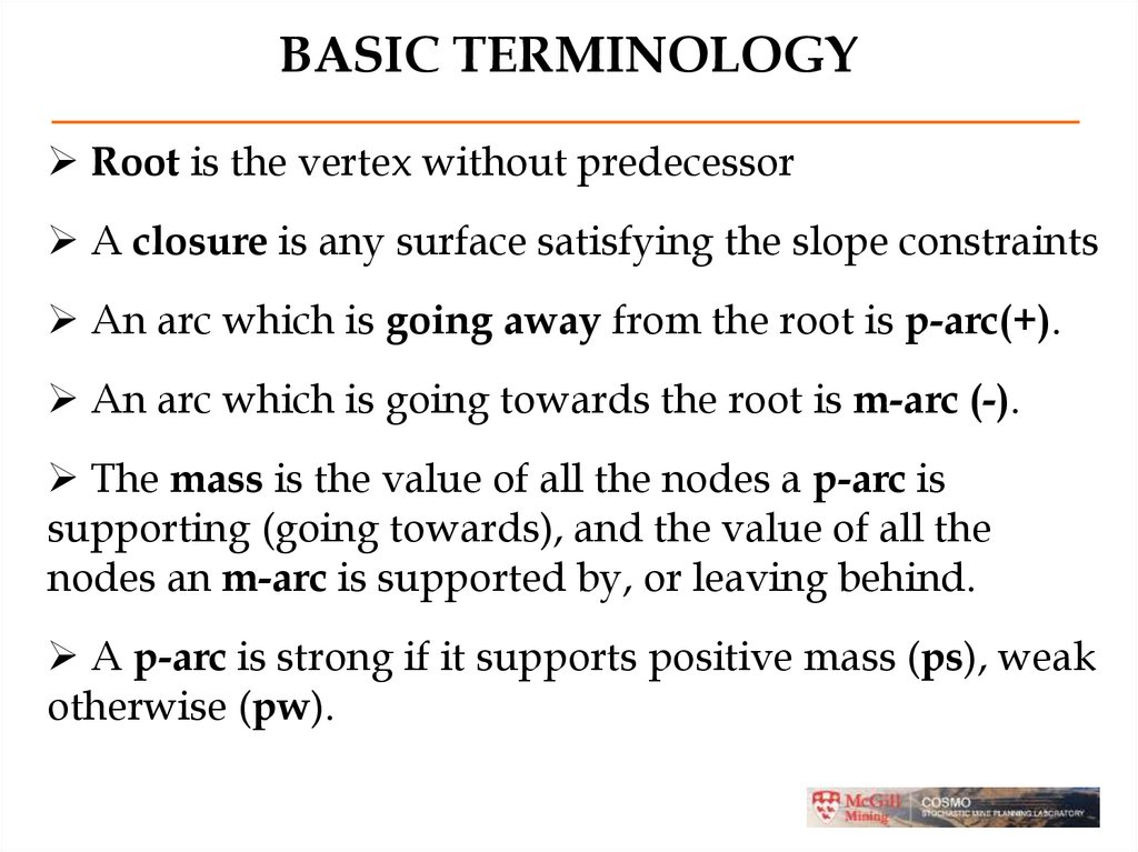
BASIC TERMINOLOGY
Root is the vertex without predecessor
A closure is any surface satisfying the slope constraints
An arc which is going away from the root is p-arc(+).
An arc which is going towards the root is m-arc (-).
The mass is the value of all the nodes a p-arc is
supporting (going towards), and the value of all the
nodes an m-arc is supported by, or leaving behind.
A p-arc is strong if it supports positive mass (ps), weak
otherwise (pw).

15.

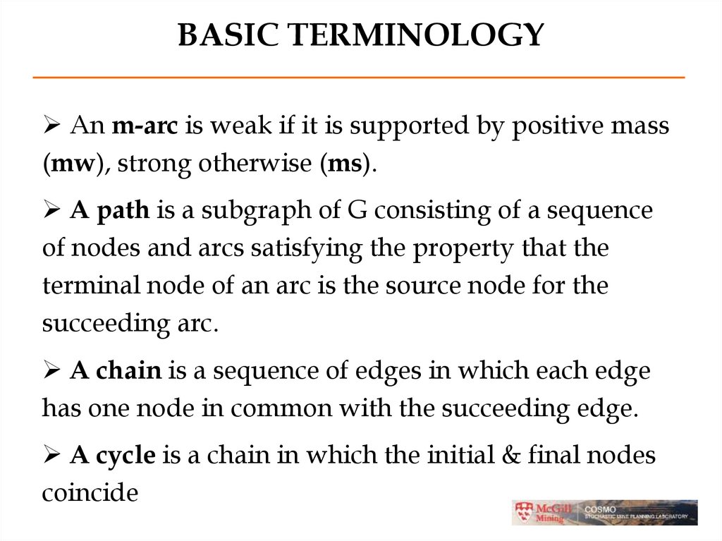
BASIC TERMINOLOGY
An m-arc is weak if it is supported by positive mass
(mw), strong otherwise (ms).
A path is a subgraph of G consisting of a sequence
of nodes and arcs satisfying the property that the
terminal node of an arc is the source node for the
succeeding arc.
A chain is a sequence of edges in which each edge
has one node in common with the succeeding edge.
A cycle is a chain in which the initial & final nodes
coincide

16.

Example of LG
-2
-2
-3
-3
-4
-2
X
-8
+6
+9
-6
X
-3
+6
+9
X0
Root node
-4

17.

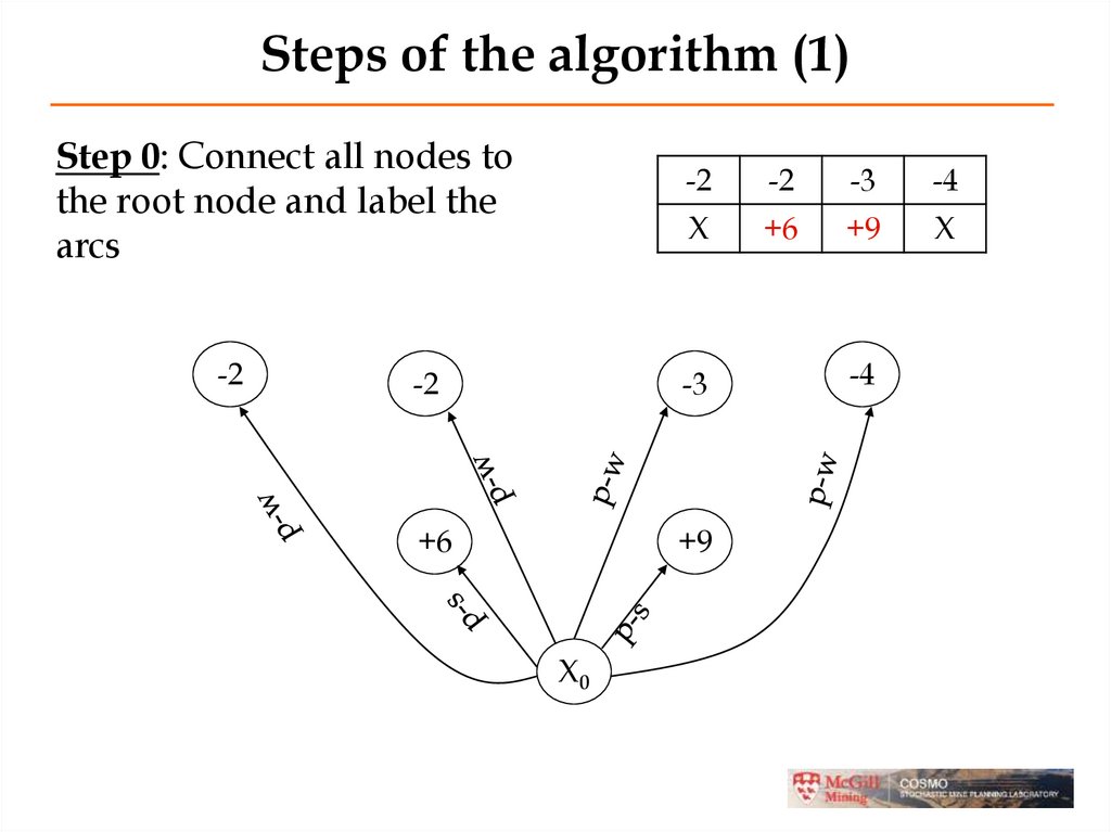
Steps of the algorithm (1)
Step 0: Connect all nodes to
the root node and label the
arcs
-2
-2
-2
-3
-4
X
+6
+9
X
-2
-3
+6
+9
X0
-4

18.

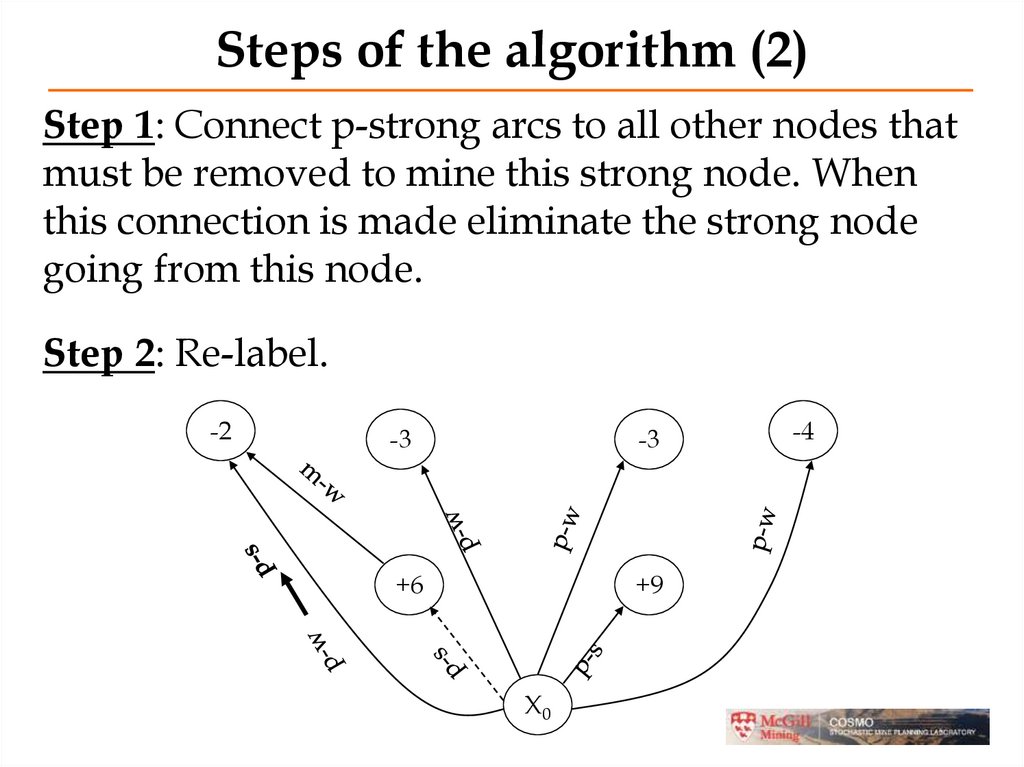
Steps of the algorithm (2)
Step 1: Connect p-strong arcs to all other nodes that
must be removed to mine this strong node. When
this connection is made eliminate the strong node
going from this node.
Step 2: Re-label.
-2
-3
-3
+6
+9
X0
-4

19.

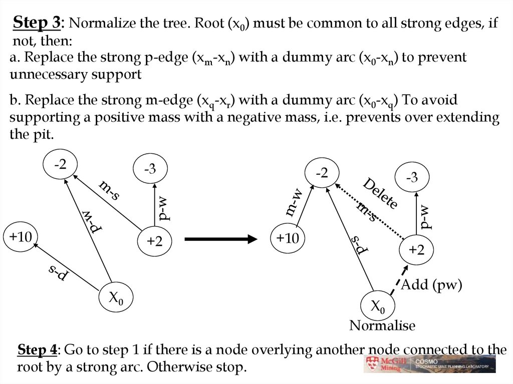
Step 3: Normalize the tree. Root (x0) must be common to all strong edges, if
not, then:
a. Replace the strong p-edge (xm-xn) with a dummy arc (x0-xn) to prevent
unnecessary support
b. Replace the strong m-edge (xq-xr) with a dummy arc (x0-xq) To avoid
supporting a positive mass with a negative mass, i.e. prevents over extending
the pit.
-2
-3
+10
+2
X0
-2
+10
-3
+2
Add (pw)
X0
Normalise
Step 4: Go to step 1 if there is a node overlying another node connected to the
root by a strong arc. Otherwise stop.

20.

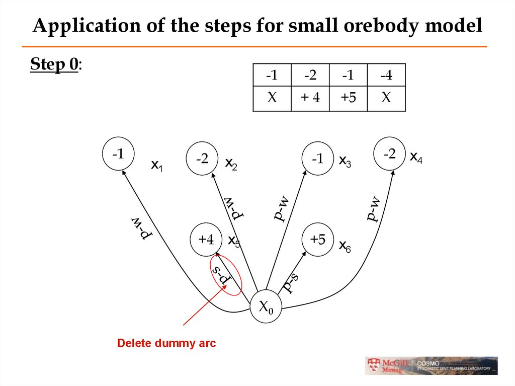
Application of the steps for small orebody model
Step 0:
-1
x1
-2
-1
-2
-1
-4
X
+4
+5
X
-1
x3
-2 x4
x2
+4 x5
+5 x
6
X0
Delete dummy arc

21.

Application of the steps …
Step 1 and 2:
-1
x1
-2
x2
-1
+4
x5
+5 x
6
delete
X0
arc (x0-x1)=-1 + 4 = +3 p-s
x3
-2
x4

22.

Application of the steps …
Step 1-2
x1
-2
x2
-1
x5
+5 x
6
x3
m-w
-1
+4
X0
arc (x0-x2)=-1 -2 + 4 = +1 p-s
-2
x4

23.

Application of the steps …
Step 1-2
-1
x2
+4
x3
pw
x1
-2
mw
-1
+5 x
6
x5
X0
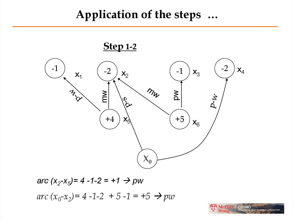
arc (x2-x5)= 4 -1-2 = +1 pw
arc (x0-x2)= 4 -1-2 + 5 -1 = +5 pw
-2
x4

24.

Application of the steps …
Step 1-2
x1
-2
-1
x2
+4
x3
pw
MW
-1
+5 x
6
x5
X0
arc (x0-x2)= 4 -1-2 + 5 -1-2= +3 p-s
-2
x4

25.

Application of the steps …
Step 1-2
x1
-2
-1
x2
+4
x3
-2
pw
MW
-1
+5 x
6
x5
Branch T26
X0
arc (x0-x2)= 4 -1-2 + 5 -1-2= +3 p-s
x4

26.

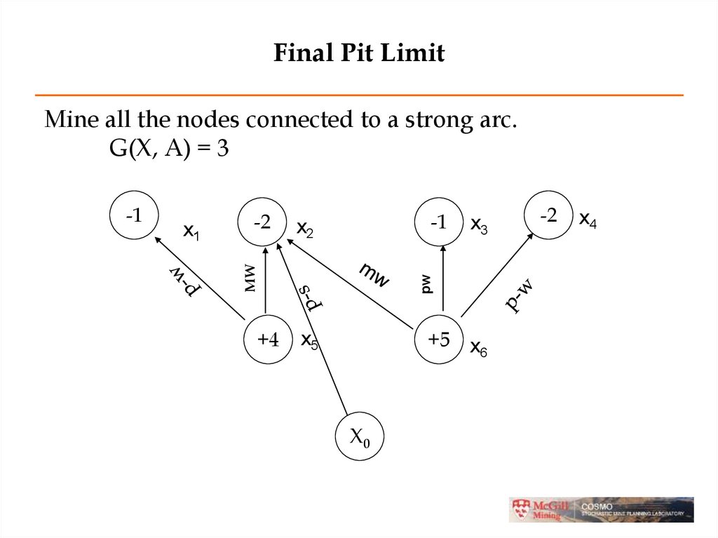
Final Pit Limit
Mine all the nodes connected to a strong arc.
G(X, A) = 3
-1
x2
+4
x3
pw
x1
-2
MW
-1
+5 x
6
x5
X0
-2
x4

27. Optimal Pit

• The L-G algorithm will flag each block as being
inside or outside the optimal pit outline
• In the 3D algorithm, the optimal pit will be the
pit with the highest net value
• Revenue can be calculated from ore tonnages,
grades, recoveries and product price.
• Price is often the biggest unknown but, in order
to design a pit, you must assume some price

28. Varying Slope Angles

• It is possible to have different slope angles in
different areas of the pit (different levels or different
X, Y coordinates)
• Results in an irregular pit wall (complete blocks
being removed)
• Bulges in the pit can lead to geotechnical concerns
• Must be corrected before the pit is complete

29. 3. Fundamental Tree Algorithm

Long-term production scheduling consists of
determining an optimal sequence of extracting the
mineralized material from the ground annualy.
MIP models are used to solve the problem for an
open pit mine.
Assume that ultimate pit and pushbacks are given
already.
Even optimizing the production schedule on a
pushback using MIP can be too complex (too
many blocks).

30. The Approach

• To simplify the MIP we would like to decrease
the number of blocks in our model so that the
MIP model can be solved efficiently.
• This is done by combining blocks that should be
mined together as just one block.
• We call the combined block a fundamental tree.

31. The Approach

A Fundamental Tree is defined as a
combination of blocks such that:
The blocks can be profitably mined.
The blocks obey the slope constraints.
There is no proper subset of the chosen blocks
that meets 1 and 2.

32. 3.1. Fundamental Tree Algorithm

33. Step 1 - Generate a Starting Network

• Given a our pushback block model represent
blocks by nodes of a graph.
• Arcs go from positive blocks to overlying
negative blocks that must be removed before
based on slope constraints.
• We will use a network flow to find the
fundamental trees.
• To construct a network flow, we add a source
node s and a sink node t.

34. Example of Generating a Starting Network

Example 2-D block model, shows the node numbers
and the block economic values in $/t
Network representation of the
2D block model, a source node s
and a sink node t are added.

35. Step 2 - Find the Cone Value

• The "cone" value of a block (CVi) is the sum of
the block values of itself and all overlying blocks
• We calculate the cone value of all positive nodes
in our pushback (or pit), CVi
Example of step 2
CV6 = V6+V1+V2+V3
=+6 — 1 — 2 — 2 = +1
CV7 = —3,
CV8 = —2

36. Step 3 – Assign cofficients to the Positive Nodes

• Each positive node will be assigned a cofficient,
Ci which denotes the rank of node i.
• Assign Ci to the nodes by ordering mining level
firstly, then by cone value.
• The maximum value on the top most level will
be given size 1 for the highest cone, and the
second highest cone value is 2 …
• With tie condition, Cis are choosen randomly

37. Example

CV6 = +1; CV7 = —3; CV8 = —2
Coefficients Ci are assigned to
positive value nodes according to
CVi value and the levels where
nodes are located.
Since CV6 > C8 > CV7, we assign
CV6 = 1
CV8 = 2
CV7 = 3

38. Step 4 - Set up the LP

• Set up a Linear Program to find the first iteration
of Fundamental Trees.
• The LP model can be solved using a
commercially availble software such as CPLEX

39. Step 5 - Check if we are done

• If the number of Fundamental Trees found is the
same as the number of trees obtained from
previous solution, go to Step 7.
• Otherwise, go to Step 6 to reformulate the
problem as a network flow and repeat. We do this
by deleting arc with no flow from our network
and resolving the new LP (go back Step 2).

40. 3.2. Formulating the Linear Program * The objective function:

n
w
i
j
Min C i f ij
Ci is the coefficient for node (block) i,
fi, j is the flow from block i to block j.
* The Flow Constraints:
1.
fs, i < Vi i where Vi > 0.
2.
fj, t = -Vj +
Oj
3.
f
i
4.
i, j
f j ,t 0
wi
f s ,i f i , j 0
j 1

41. Example of Step 4

CV6 = 1
CV8 = 2
CV7 = 3
Minimise
f61+f62+f63+3f72+3f73+3f74 +2f83+2f84+2f85
Subject To
Variable
fs6 <= 6
fS6
5.003000
fs7 <= 3
fS7
0.002000
fs8 <= 4
fS8
4.000000
f 1t = 1.001
f1t
1.001000
f2t= 2.001
f2t
2.001000
f3t = 2.001
f3t
2.001000
f4t= 2.001
f4t
2.001000
f5t = 2.001
f5t
2.001000
f61-f1t= 0
f61
1.001000
f62+f72-f2t = 0
f62
2.001000
f63+f73+f83-f 3t = 0
f63
2.001000
f74+f84-f4t = 0
f72
00000
f85-f5t = 0
f73
0.000000
fs6-f61-f62-f63 = 0
f74
0.002000
fs7-f72-f73-f74 = 0
f83
0.000000
fs8-f83-f84-f85 = 0
f84
1.999000
f85
2.001000
Value

42. Example of Step 4

The network representation of the
initial solution containing two trees
surrounded by dashed lines.

43. Example of Step 4

Minimise
f61+f62+f63+2 f74 +3f84+ 3f85
Subject To
Variable
Value
fs6 <= 6
fS6
5.003000
fs7 <= 3
fS7
2.001000
fs8 <= 4
fS8
2.001000
f1t = 1.001
f1t
1.001000
f2t = 2.001
f2t
2.001000
f3t = 2.001
f3t
2.001000
f4t = 2.001
f4t
2.001000
f5t = 2.001
f5t
2.001000
f61-f1t= 0
f61
1.001000
f62 -f2t= 0
f62
2.001000
f63 -f3t = 0
f63
2.001000
f74+f84-f4t = 0
f74
2.001000
f85-f5t= 0
f84
0.000000
fs6-f61-f62-f63 = 0
f85
2.001000
fs7 -f74 = 0
fs8 -f84-f85 = 0
The network representation the
solution containing three trees
surrounded by dashed lines.

44. 3.3. Properties of the fundamental trees

• Property 1 - All fundamental trees have positive
value is satisfied since: Vi f s , j
i
( V ) f
and
j
j
i
s, j
i
Therefore,
V ( V )
i
i
j
j
• The sum of all positive value nodes in a tree is
greater than the sum of negative value nodes.

45. Property 2 of the fundamental trees

• All fundamental trees obey the slope constraints
if they are removed one at a time respecting the
sequencing between them.
• All overlying negative nodes must be supported
by positive nodes by the LP constraints.

46. Property 3 of the fundamental trees

• A tree found by FTcannot contain a subset
of a fundamental tree that also can be a
fundamental tree.
Base on the objective function,
C f
i
i
i, j
j
• Where i nodes are positive and j nodes are
negative, if a smaller fundamental tree
existed then our LP would have found it.

47. 3.4. Optimization of annual production scheduling using fundamental trees

• The optimization model is maximization of the
NPV, or discounted economic value, to be
generated from the mining operation
• For scheduling N Fundamental Trees over Y
years, the objective function can be expressed as:
Y
N
Max ( DEV pi ) * Oip ( DWC pi * Wip
p 1 i 1

48. using fundamental trees

• Where:
DEVpi discounted economic value to be feberated from
mining and processing all the ore tons in year, p from FTi,
DEVpi = DEV0i*DFp
(DFp = 1/(1.0 + d)p
DWCip discounted average cost of mining one ton waste
from FTi in year p, DWCip = DWCi0*DFp
Wip is a linear variable representing the tons of the waste to
be mined at period p from fundamental tree i
Oip is a binary variable, equal to 1 if the ore ton in FTi is
scheduling for period p, 0 otherwise.

49.

Subject to:
. Slope constraints:
If j is the index for the fundamental trees that have to
be removed before being able to remove tree i in a
period p:
p
Oip O jt 0
t 1
If Ni is the number of overlying FTs for FT i:
Ni
p
j
t 1
N i Oip Ojt 0

50.

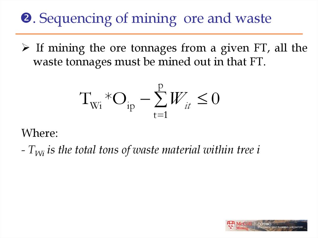
. Sequencing of mining ore and waste
If mining the ore tonnages from a given FT, all the
waste tonnages must be mined out in that FT.
p
TWi *Oip Wit 0
t 1
Where:
- TWi is the total tons of waste material within tree i

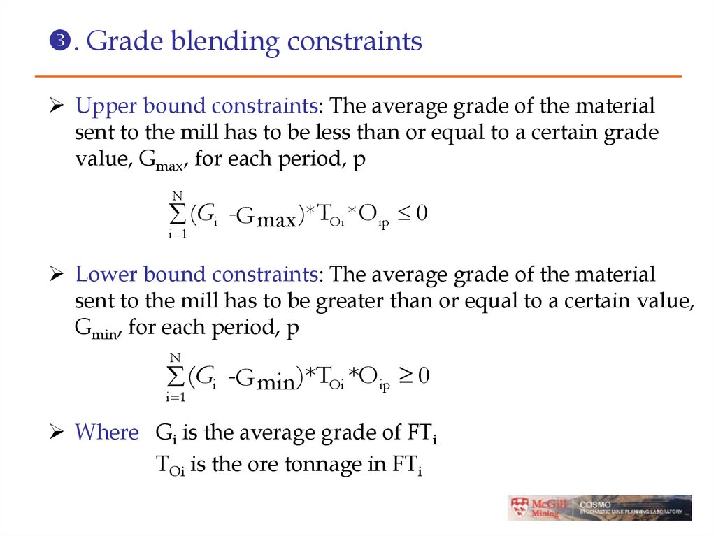
51.

. Grade blending constraints
Upper bound constraints: The average grade of the material
sent to the mill has to be less than or equal to a certain grade
value, Gmax, for each period, p
N
(Gi -G max )*TOi *O ip 0
i 1
Lower bound constraints: The average grade of the material
sent to the mill has to be greater than or equal to a certain value,
Gmin, for each period, p
N
(Gi -G min )*TOi *Oip 0
i 1
Where Gi is the average grade of FTi
TOi is the ore tonnage in FTi

52.

. Processing capacity constraints
Upper bound: The total tonnage of ore
processed cannot be more than the processing
capacity (PCmax) in any period, p
N
(T *O ) PC
i 1
Oi
ip
max
Lower bound: The total tonnage of ore
processed cannot be less than a certain amount
(PCmin) in any period, p
N
(T *O ) PC
i 1
Oi
ip
min

53.

. Reserve constraints
Y
Oip 1
p 1
. The limit on the stripping ratio in each period
N
(W SR
ip
i 1
+
max
* TOi O ip ) 0
Where
SRmax is the maximum stripping ratio allowed during any year

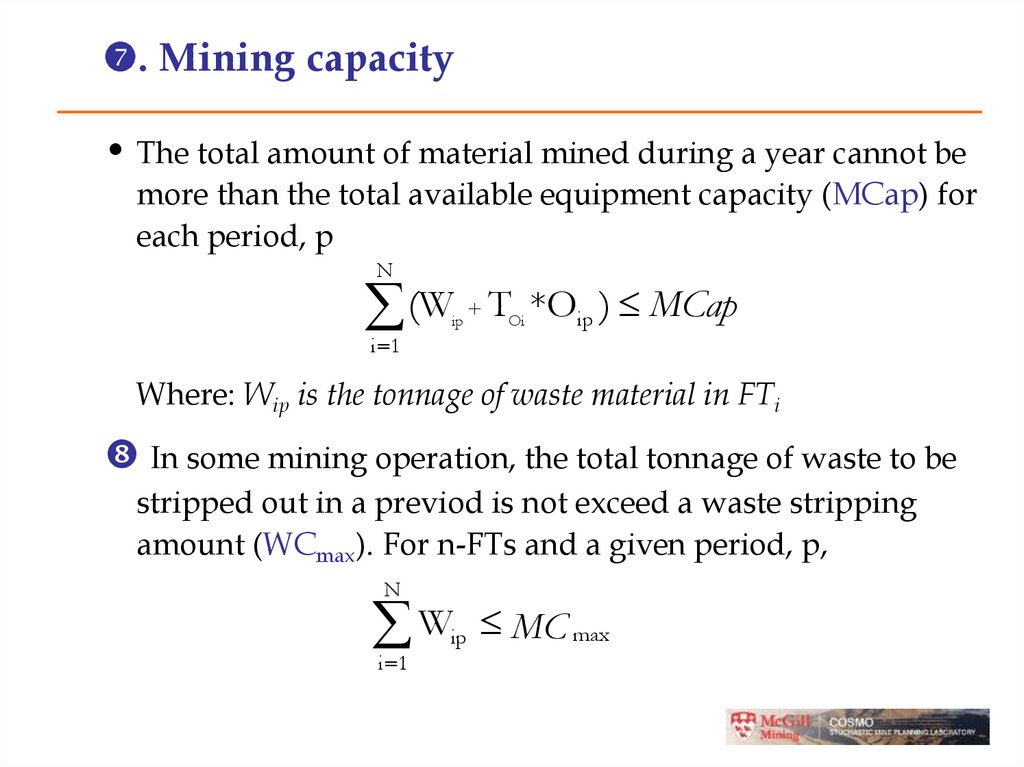
54.

. Mining capacity
• The total amount of material mined during a year cannot be
more than the total available equipment capacity (MCap) for
each period, p
N
(W T *O ) MCap
ip
+
Oi
i 1
ip
Where: Wip is the tonnage of waste material in FTi
In some mining operation, the total tonnage of waste to be
stripped out in a previod is not exceed a waste stripping
amount (WCmax). For n-FTs and a given period, p,
N
W MC
i 1
ip
max

55. 3.5. Case Study: MIP Scheduling Formulation

• One of the case studies is performed on a large
copper mine in Southern Peru containing 1 million
blocks
• MIP formulations for mine scheduling treating
fundamental trees as single blocks.
• This algorithm reduced the number of blocks from
38457 to 5512 fundamental trees.
• Therefore, large open pit production scheduling can
be optimized by MIP modelling for any objective
such as maximizing NPV of a given mine project, or
to solve hard ore quality and grade blending
problems

56. ASSIGNMENT 8

j
1
2
3
4
5
6
7
1
-2
-2
-3
-3
-4
-2
-2
2
-3
+5
+7
-1
+8
+4
-4
3
-4
-3
-4
+6
+3
-4
-5
i
Consider the above 2D orebody model:
1. Show steps to determine the ultimate pit limits using:
a) Cone mining algorithm (if known)
b) LG algorithm (Dynamic Programming) (if known)
c) LG algorithm (Graph closure)
Describe the differences between the algorithms.
2. Write codes in C++ to solve the above problem using Graph closure (LG)

57. ASSIGNMENT 8

3. Suppose that we have 2 D section below, show your result obtaining from
running your program (C++ code)
-4
-4
-4
-4
-4
8
12
12
0
-4
-4
-4
-4
-4
-4
-4
-4
-4
-4
-4
-4
-4
-4
-4
0
12
12
8
-4
-4
-4
-4
-4
-4
-4
-4
-4
-4
-4
-4
-4
-4
-4
-4
8
12
12
0
-4
-4
-4
-4
-4
-4
-4
-4
-4
-4
-4
-4
-4
-4
-4
0
12
12
8
-4
-4
-4
-4
-4
-4
-4
-4
-4
-4
-4
-4
-4
-4
-4
-4
10
12
12
0
-4
-4
-4
-4
-4
-4
-4
-4
-4
-4
-4
-4
-4
-4
-4
0
12
12
7
-4
-4
-4
-4
-4
-4
-4
-4
-4
-4
-4
-4
-4
-4
-4
-4
8
12
12
0
-4
-4
-4
-4
-4
-4
-4
-4
-4
-4
-4
-4
-4
-4
-4
0
12
12
9
-4
-4
-4
-4
-4
-4
-4
-4
-4
-4
-4
-4
-4
-4
-4
-4
12
12
12
5
-4
-4
-4
-4
-4
-4