Elements of chance: probability methods statistics for business and economics

1.

ELEMENTS OF CHANCE:
PROBABILITY METHODS
STATISTICS FOR BUSINESS AND ECONOMICS 13e Anderson,
David R 2017

2.

Introduction to Probability
RANDOM
EXPERIMENTS
EVENTS AND THEIR
PROBABILITIES
BASIC
RELATIONSHIPS OF
PROBABILITY
CONDITIONAL
PROBABILITY
BAYES’ THEOREM

3.

Statistics in Practice
■ Responsible for the US civilian space program and aeronautics and aerospace
research
■ Best known for its manned space exploration. Motto: “pioneer the future in space
exploration, scientific discovery and aeronautics research”
■ Currently working on “Space Launch System” that will the astronauts farther into
space than ever before
■ Although NASA’s primary mission is space exploration, its expertise has been called
upon to assist countries and organizations throughout the world

4.

Statistics in Practice
■ In one such situation in San Jose
■ Gold mine in Copiapo, Chile, caved in, trapping 33 men more than 2000 feet
underground
■ Issue: although it was primary importance to bring men safely to the surface as
quickly as possible, it was imperative that the rescue effort be carefully designed and
implemented to save as many miners as possible
■ The Chilean government asked NASA for help to provide assistance in developing a
rescue method

5.

Statistics in Practice
■ NASA sent a four-person team consisting of an engineer, two physicians and a
psychologist with expertise in vehicle design and issues of long-term confinement
■ The probability of success and failure of various rescue methods was prominent in
the thoughts of everyone involved
■ Since there were no historical data available that applied to this unique rescue
situation, NASA scientists developed subjective probability estimates from the success
and failure of various rescue methods based on similar circumstances experienced by
astronauts from short- and long-term space missions

6.

Statistics in Practice
■ The probability estimates provided by Nasa guided officials in the selection of a
rescue method and provided insight as to how the miners would survive the ascent
in a rescue cage.
■ The rescue method designed by the Chilean officials in consultation with the Nasa
team resulted in the construction of 13-foot-long, 924-pound steel rescue capsule
that would be used to bring up the miners one at a time.
■ All miners were rescued, with the last miner emerging 68 days after the cave-in
occurred.

7.

Statistics in Practice
■ In this chapter you will learn about probability as well as how to compute and
interpret probabilities for a variety of situations.
■ In addition to subjective probabilities, you will learn about classical and relative
frequency methods for assigning probabilities. the basic relationships of probability,
conditional probability, and Bayes’ theorem will be covered.

8.

1. Random Experiments, Counting
Rules, and Assigning Probabilities
Probability
■ Numerical measure of the likelihood that an event will occur
■ Managers often base their decisions on an analysis of uncertainties such as the
following:
– What are the chances that sales will decrease if we increase prices?
– What is the likelihood a new assembly method will increase productivity?
– How likely is it that the project will be finished on time?
– What is the chance that a new investment will be profitable?

9.

1. Random Experiments, Counting
Rules, and Assigning Probabilities
Probability
■ Probabilities can be used as measures of the degree of
■ If probabilities are available, we can determine the likelihood of each event
occurring.
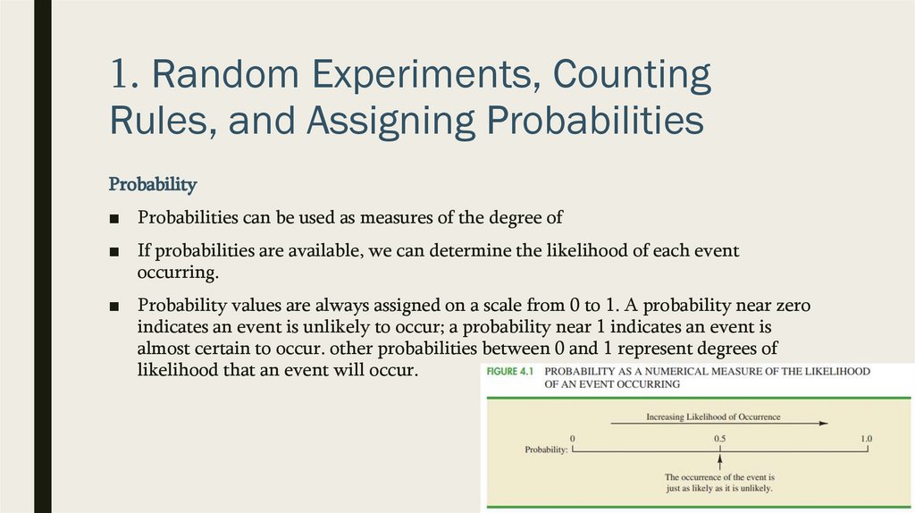
■ Probability values are always assigned on a scale from 0 to 1. A probability near zero
indicates an event is unlikely to occur; a probability near 1 indicates an event is
almost certain to occur. other probabilities between 0 and 1 represent degrees of
likelihood that an event will occur.

10.

1. Random Experiments, Counting
Rules, and Assigning Probabilities
Random Experiments
■ In discussing probability, we deal with experiments that have the following
characteristics:
– The experimental outcomes are well defined, and in many cases can even be
listed prior to conducting the experiment.
– On any single repetition or trial of the experiment, one and only one of the
possible experimental outcomes will occur.
– The experimental outcome that occurs on any trial is determined solely by
chance.

11.

1. Random Experiments, Counting
Rules, and Assigning Probabilities
Random Experiments
■ Defined as:

12.

1. Random Experiments, Counting
Rules, and Assigning Probabilities
Random Experiments
■ To illustrate the key features associated with a random
experiment, consider the process of tossing a coin.
– two possible experimental outcomes: head or tail
– only one of the two possible experimental outcomes
will occur
– the outcome that occurs on any trial is determined
solely by chance or random variability

13.

1. Random Experiments, Counting
Rules, and Assigning Probabilities
Sample space
■ The sample space for a random experiment is the set of all experimental outcomes
■ Examples
– Tossing a coin
– Rolling a die

14.

1. Random Experiments, Counting
Rules, and Assigning Probabilities
Counting Rules
■ Multi-step experiments
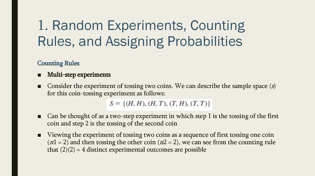
■ Consider the experiment of tossing two coins. We can describe the sample space (s)
for this coin-tossing experiment as follows:
■ Can be thought of as a two-step experiment in which step 1 is the tossing of the first
coin and step 2 is the tossing of the second coin
■ Viewing the experiment of tossing two coins as a sequence of first tossing one coin
(n1 = 2) and then tossing the other coin (n2 = 2), we can see from the counting rule
that (2)(2) = 4 distinct experimental outcomes are possible

15.

1. Random Experiments, Counting
Rules, and Assigning Probabilities
Counting Rules
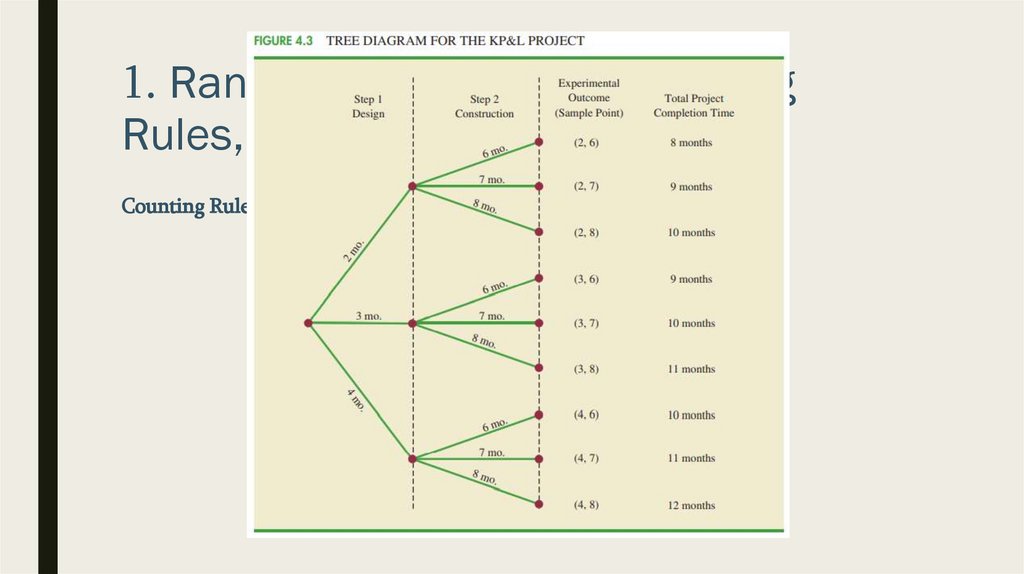
■ We can construct a tree diagram,
graphical representation that helps
visualizing a multi-step experiment

16.

1. Random Experiments, Counting
Rules, and Assigning Probabilities
Counting Rules
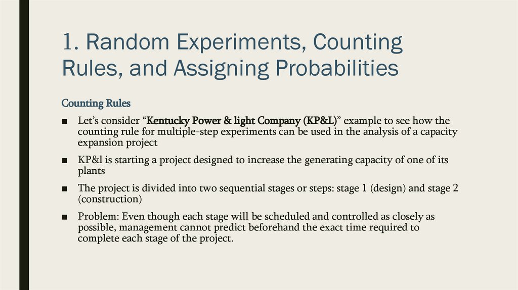
■ Let’s consider “Kentucky Power & light Company (KP&L)” example to see how the
counting rule for multiple-step experiments can be used in the analysis of a capacity
expansion project
■ KP&l is starting a project designed to increase the generating capacity of one of its
plants
■ The project is divided into two sequential stages or steps: stage 1 (design) and stage 2
(construction)
■ Problem: Even though each stage will be scheduled and controlled as closely as
possible, management cannot predict beforehand the exact time required to
complete each stage of the project.

17.

1. Random Experiments, Counting
Rules, and Assigning Probabilities
Counting Rules
■ An analysis of similar construction projects revealed possible completion times for
– The design stage of 2, 3, or 4 months
– and possible completion times for the construction stage of 6, 7, or 8 months.
■ In addition, because of the critical need for additional electrical power, management
set a goal of 10 months for the completion of the entire project.
■ Is it a reasonable goal? Why 10 and not 9 or 11?

18.

1. Random Experiments, Counting
Rules, and Assigning Probabilities
Counting Rules
■ Three possible completion times for the design stage (step 1)
■ And three possible completion times for the construction stage (step 2)
■ The counting rule for multiple-step experiments can be applied here to determine a
total of (3)(3) = 9 experimental outcomes.
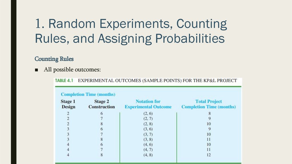
■ To describe the experimental outcomes, we use a two-number notation; for instance,
(2, 6) indicates that the design stage is completed in 2 months and the construction
stage is completed in 6 months. This experimental outcome results in a total of 2 + 6
= 8 months to complete the entire project.

19.

1. Random Experiments, Counting
Rules, and Assigning Probabilities
Counting Rules
■ All possible outcomes:

20.

1. Random Experiments, Counting
Rules, and Assigning Probabilities
Counting Rules

21.

1. Random Experiments, Counting
Rules, and Assigning Probabilities
Counting Rules
■ We see that the project will be completed in 8 to 12 months
■ Six of the nine experimental outcomes providing the desired completion time of 10
months or less
■ Even though identifying the experimental outcomes may be helpful, we need to
consider how probability values can be assigned to the experimental outcomes before
making an assessment of the probability that the project will be completed within
the desired 10 months.

22.

1. Random Experiments, Counting
Rules, and Assigning Probabilities
Combination
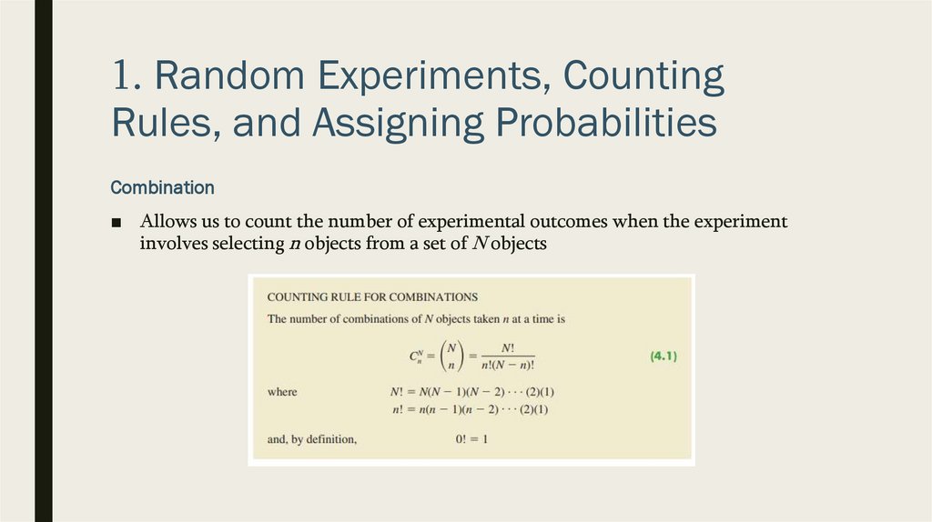
■ Allows us to count the number of experimental outcomes when the experiment
involves selecting n objects from a set of N objects

23.

1. Random Experiments, Counting
Rules, and Assigning Probabilities
Combination
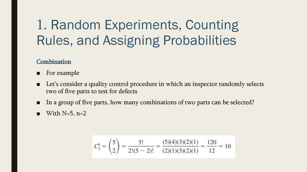
■ For example
■ Let’s consider a quality control procedure in which an inspector randomly selects
two of five parts to test for defects
■ In a group of five parts, how many combinations of two parts can be selected?
■ With N=5, n=2

24.

1. Random Experiments, Counting
Rules, and Assigning Probabilities
Combination
■ Thus, 10 outcomes are possible for the experiment of randomly selecting two parts
from a group of five.
■ If we label the five parts as A, b, C, D, and E, the 10 combinations or experimental
outcomes can be identified as

25.

1. Random Experiments, Counting
Rules, and Assigning Probabilities
Combination
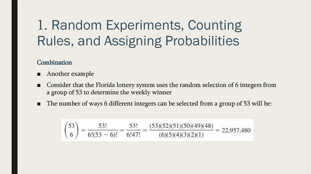
■ Another example
■ Consider that the Florida lottery system uses the random selection of 6 integers from
a group of 53 to determine the weekly winner
■ The number of ways 6 different integers can be selected from a group of 53 will be:

26.

1. Random Experiments, Counting
Rules, and Assigning Probabilities
Permutations
■ It allows one to compute the number of experimental outcomes when n objects are
to be selected from a set of N objects where the order of selection is important.

27.

1. Random Experiments, Counting
Rules, and Assigning Probabilities
Permutations
■ For example
■ Let’s consider again the quality control process in which an inspector selects two of
five parts to inspect for defects. how many permutations may be selected?
■ With n = 5 and n = 2, we have
■ If we label the parts A, b, C, D, and E, the 20 permutations are

28.

1. Random Experiments, Counting
Rules, and Assigning Probabilities
Assigning Probabilities
■ Now let us see how probabilities can be assigned to experimental outcomes. The
three approaches most frequently used are:
– the classical,
– relative frequency,
– and subjective methods

29.

1. Random Experiments, Counting
Rules, and Assigning Probabilities
Assigning Probabilities
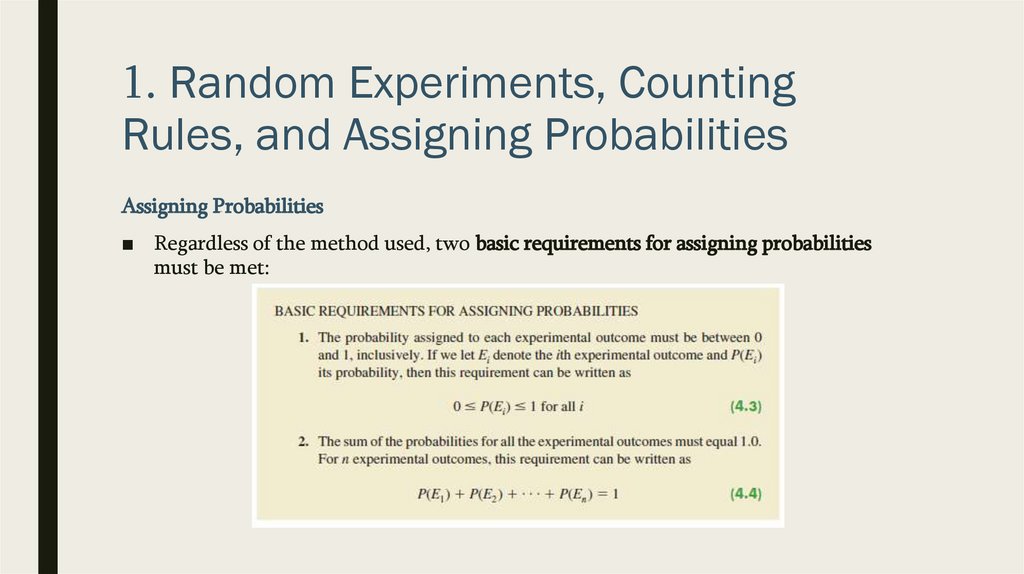
■ Regardless of the method used, two basic requirements for assigning probabilities
must be met:

30.

1. Random Experiments, Counting
Rules, and Assigning Probabilities
Assigning Probabilities
■ The Classical Method
■ Assigning probabilities is appropriate when all the experimental outcomes are
equally likely
■ If n experimental outcomes are possible, a probability of 1/n is assigned to each
experimental outcome
■ For an example, consider the experiment of tossing a fair coin; the two experimental
outcomes—head and tail—are equally likely.
■ Because one of the two equally likely outcomes is a head, the probability of
observing a head is 1/2, or .50.
■ Similarly, the probability of observing a tail is also 1/2, or .50

31.

1. Random Experiments, Counting
Rules, and Assigning Probabilities
Assigning Probabilities
■ The Relative Frequency Method
■ Assigning probabilities is appropriate when data are available to estimate the
proportion of the time the experimental outcome will occur if the experiment is
repeated a large number of times.
■ As an example, consider a study of waiting times in the X-ray department for a local
hospital.

32.

1. Random Experiments, Counting
Rules, and Assigning Probabilities
Assigning Probabilities
■ The Relative Frequency Method
■ A clerk recorded the number of patients waiting for
service at 9:00 a.m. on 20 successive days and
obtained the following results
■ Using the relative frequency method, we would
assign a probability of 2/20 = .10 to the experimental
outcome of zero patients waiting for service, 5/20 =
.25 to the experimental outcome of one patient
waiting, etc.

33.

1. Random Experiments, Counting
Rules, and Assigning Probabilities
Assigning Probabilities
■ The Subjective Method
■ Assigning probabilities is most appropriate when one cannot realistically assume that
the experimental outcomes are equally likely and when little relevant data are
available.
■ When the subjective method is used to assign probabilities to the experimental
outcomes, we may use any information available, such as our experience or
intuition.
■ After considering all available information, a probability value that expresses our
degree of belief (on a scale from 0 to 1) that the experimental outcome will occur is
specified. because subjective probability expresses a person’s degree of belief, it is
personal.
■ Using the subjective method, different people can be expected to assign different
probabilities to the same experimental outcome

34.

1. Random Experiments, Counting
Rules, and Assigning Probabilities
Assigning Probabilities
■ The Subjective Method
■ Consider the case in which Tom and Judy Elsbernd make an offer to purchase a
house. Two outcomes are possible:
– E1 = their offer is accepted
– E2 = their offer is rejected

35.

1. Random Experiments, Counting
Rules, and Assigning Probabilities
Assigning Probabilities
■ The Subjective Method
■ Judy believes that the probability their offer will be accepted is .8; thus, Judy would set
■ P(E1) = .8 and P(E2) = .20
■ Tom, however, believes that the probability that their offer will be accepted is .6; hence,
Tom would set P(E1) = .6 and P(E2) = .40
■ Note that Tom’s probability estimate for E1 reflects a greater pessimism that their offer
will be accepted.
■ Both Judy and Tom assigned probabilities that satisfy the two basic requirements. The
fact that their probability estimates are different emphasizes the personal nature of the
subjective method.

36.

1. Random Experiments, Counting
Rules, and Assigning Probabilities
Assigning Probabilities
■ The Subjective Method
■ Even in business situations where either the classical or the relative frequency
approach can be applied, managers may want to provide subjective probability
estimates.
■ In such cases, the best probability estimates often are obtained by combining the
estimates from the classical or relative frequency approach with subjective
probability estimates.

37.

1. Random Experiments, Counting
Rules, and Assigning Probabilities
Assigning Probabilities
■ KP&L Project
■ Let’s perform further analysis
■ We must develop probabilities for each of the nine experimental outcomes
■ On the basis of experience and judgment, management concluded that the
experimental outcomes were not equally likely. Hence, the classical method of
assigning probabilities could not be used
■ Management then decided to conduct a study of the completion times for similar
projects undertaken by KP&l over the past three years.
■ Let’s take a look at a study of 40 similar projects

38.

1. Random Experiments, Counting
Rules, and Assigning Probabilities
Assigning Probabilities
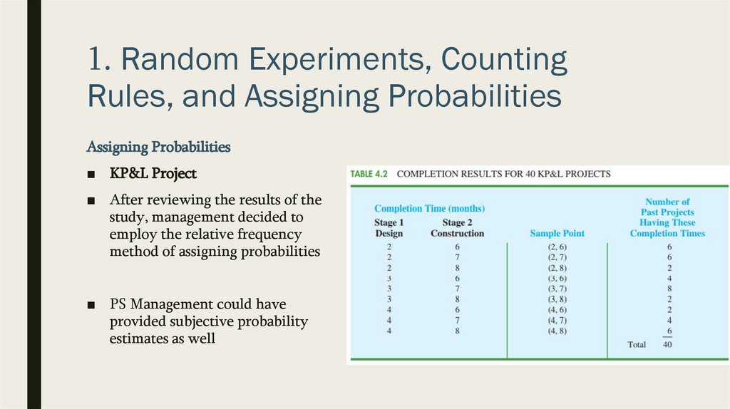
■ KP&L Project
■ After reviewing the results of the
study, management decided to
employ the relative frequency
method of assigning probabilities
■ PS Management could have
provided subjective probability
estimates as well

39.

1. Random Experiments, Counting
Rules, and Assigning Probabilities
Assigning Probabilities
■ KP&L Project

40.

2. Events and Their Probabilities
An Event
■ An event is a collection of sample points
■ KP&L Project example
– Project manager is interested in the event that the entire project can be
completed in 10 months or less
– We see that six sample points—(2, 6), (2, 7), (2, 8), (3, 6), (3, 7), and (4, 6)—
provide a project completion time of 10 months or less
– Let C denote the event that the project is completed in 10 months or less; we
write

41.

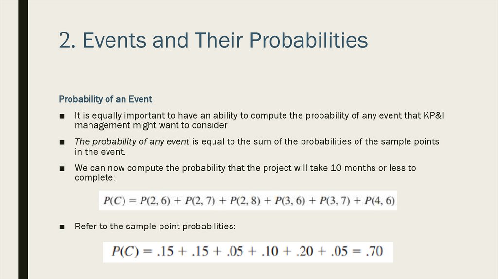
2. Events and Their Probabilities
Probability of an Event
■ It is equally important to have an ability to compute the probability of any event that KP&l
management might want to consider
■ The probability of any event is equal to the sum of the probabilities of the sample points
in the event.
■ We can now compute the probability that the project will take 10 months or less to
complete:
■ Refer to the sample point probabilities:

42.

2. Events and Their Probabilities
Probability of an Event
■ Using these probability results, we can now tell KP&l management that
– There is a .70 probability that the project will be completed in 10 months or
less,
– A .40 probability that the project will be completed in less than 10 months,
– And a .30 probability that the project will be completed in more than 10
months.

43.

3. Some Basic Relationships of
Probability
Complement of an Event
■ Venn diagram, illustrating the concept of a complement

44.

3. Some Basic Relationships of
Probability
Complement of an Event
■ Defined by formula:
■ As an example, consider the case of a sales manager who, after reviewing sales
reports, states that 80% of new customer contacts result in no sale.
■ By allowing A to denote the event of a sale:

45.

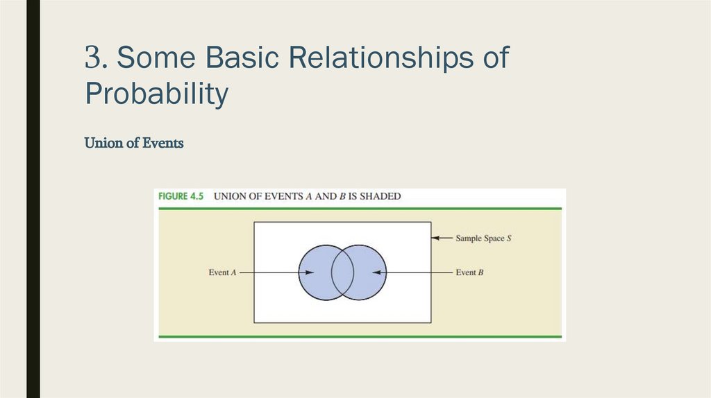
3. Some Basic Relationships of
Probability
Union of Events
■ We may be interested in knowing the probability that at least one of two events
occurs.
■ That is, with events A and B we are interested in knowing the probability that event
A or event B or both occur

46.

3. Some Basic Relationships of
Probability
Union of Events

47.

3. Some Basic Relationships of
Probability
Intersection of Two Events
■ Definition:

48.

3. Some Basic Relationships of
Probability
Addition Law
■ Provides a way to compute the probability that event A or event B or both occur:

49.

3. Some Basic Relationships of
Probability
Addition Law
■ Let us consider the case of a small assembly plant with 50 employees.
■ At the end of a performance evaluation period, the production manager found out
that
– 5 of the 50 workers completed work late,
– 6 of the 50 workers assembled a defective product,
– And 2 of the 50 workers both completed work late and assembled a defective
product
■ Let
– L = the event that the work is completed late
– D = the event that the assembled product is defective

50.

3. Some Basic Relationships of
Probability
Addition Law
■ Mutually Exclusive Events
■ Two events are said to be mutually exclusive if the events have no sample points in
common

51.

4. Conditional Probability
■ Often, the probability of an event is influenced by whether a related event already
occurred
■ Suppose we have an event A with probability P(A). If we obtain new information
and learn that a related event, denoted by B, already occurred, we will want to
■ take advantage of this information by calculating a new probability for event A.
■ This new probability of event a is called a conditional probability and is written
■ We use the notation ∣ to indicate that we are considering the probability of event a
given the condition that event B has occurred. hence, the notation P(a ∣ B) reads “the
probability of A given B.”

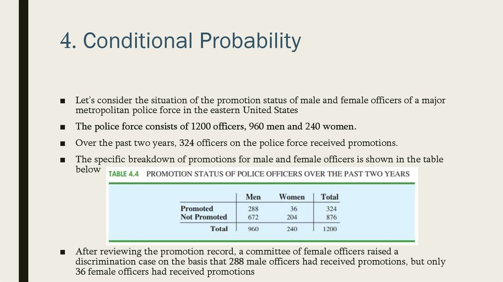
52.

4. Conditional Probability
■ Let’s consider the situation of the promotion status of male and female officers of a major
metropolitan police force in the eastern United States
■ The police force consists of 1200 officers, 960 men and 240 women.
■ Over the past two years, 324 officers on the police force received promotions.
■ The specific breakdown of promotions for male and female officers is shown in the table
below
■ After reviewing the promotion record, a committee of female officers raised a
discrimination case on the basis that 288 male officers had received promotions, but only
36 female officers had received promotions

53.

4. Conditional Probability
■ The police administration argued that the relatively low number of promotions for
female officers was due not to discrimination, but to the fact that relatively few
females are members of the police force. let us show how conditional probability
could be used to analyze the discrimination charge.
■ Let
–
–
–
–
M = event an officer is a man
W = event an officer is a woman
A = event an officer is promoted
Ac = event an officer is not promoted

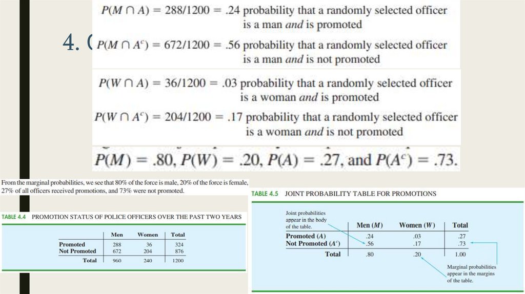
54.

4. Conditional Probability

55.

4. Conditional Probability
■ let us begin the conditional probability analysis by computing the probability that an
officer is promoted given that the officer is a man. In conditional probability
notation, we are attempting to determine P(A ∣ M)
■ P(A ∣ M) tells us that we are now concerned only with the promotion status of the
960 male officers. Because 288 of the 960 male officers received promotions, the
probability of being promoted given that the officer is a man is 288/960 = .30
■ P(A ∣ M) can be computed directly from related event probabilities rather than the
frequency data

56.

4. Conditional Probability
■ The fact that conditional
probabilities can be computed as
the ratio of a joint probability to a
marginal probability provides the
following general formula for
conditional probability
calculations for two events A and
B

57.

4. Conditional Probability
■ Independent Events
■ In our case:
■ We see that the probability of a promotion (event a) is affected or influenced by
whether the officer is a man or a woman.
■ Particularly, because P(A ∣ M) ≠ P(a), we would say that events A and M are
dependent events.
■ That is, the probability of event A (promotion) is altered or affected by knowing that
event M (the officer is a man) exists

58.

4. Conditional Probability
■ Independent Events
■ However, if the probability of event A is not changed by the existence of event M—
that is, P(a ∣ M) = P(a)—we would say that events A and M are independent events.
■ This situation leads to the following definition of the independence of two events.

59.

4. Conditional Probability
■ Multiplication Law
■ Whereas the addition law of probability is used to compute the probability of a
union of two events, the multiplication law is used to compute the probability of the
intersection of two events

60.

4. Conditional Probability
■ Multiplication Law
■ To illustrate the use of the multiplication law, consider a newspaper circulation
department where it is known that 84% of the households in a particular
neighborhood subscribe to the daily edition of the paper.
■ If we let D denote the event that a household subscribes to the daily edition, P(D) =
.84
■ In addition, it is known that the probability that a household that already holds a
daily subscription also subscribes to the Sunday edition (event S) is .75; that is, P(S ∣
D) = .75
■ What is the probability that a household subscribes to both the Sunday and daily
editions of the newspaper?
■ Using the multiplication law, we compute the desired P(S ∩ D) as

61.

4. Conditional Probability
■ Multiplication Law for Independent Events
■ For the special case of independent events, we obtain the following multiplication
law

62.

5. Bayes’ Theorem
■ In the discussion of conditional probability, we indicated that revising probabilities
when new information is obtained is an important phase of probability analysis
■ Methodology used
■ Let’s do an illustration

63.

5. Bayes’ Theorem
■ Consider a manufacturing firm that receives shipments of parts from two different
suppliers A1
■ let A1 denote the event that a part is from supplier 1 and A2 denote the event that a
part is from supplier 2.
■ Currently, 65% of the parts purchased by the company are from supplier 1 and the
remaining 35% are from supplier 2.
■ Hence, if a part is selected at random, we would assign the prior probabilities P(a1) =
.65 and P(a2) = .35
■ Historical data suggest that the quality ratings of the two suppliers are as shown
below

64.

5. Bayes’ Theorem
■ If we let G denote the event that a part is good and B denote the event that a part is
bad, then
■ We see that four experimental outcomes are possible; two correspond to the part
being good and two correspond to the part being bad:

65.

5. Bayes’ Theorem
■ Each of the experimental outcomes is the intersection of two events, so we can use
the multiplication rule to compute the probabilities

66.

5. Bayes’ Theorem
■ Suppose now that the parts from the two suppliers are used in the firm’s
manufacturing process and that a machine breaks down because it attempts to
process a bad part
■ Given the information that the part is bad, what is the probability that it came from
supplier 1 and what is the probability that it came from supplier 2?

67.

5. Bayes’ Theorem

68.

Thank You!