Financial Theory Microstructure of Financial Markets

1. Financial Theory Microstructure of Financial Markets (part 2) Topic: Market Microstructure Models International College for

Economics and Finance (ICEF)
Moscow
Seminar Lead: Alexei Boulatov
Fall 2023

2. Introduction

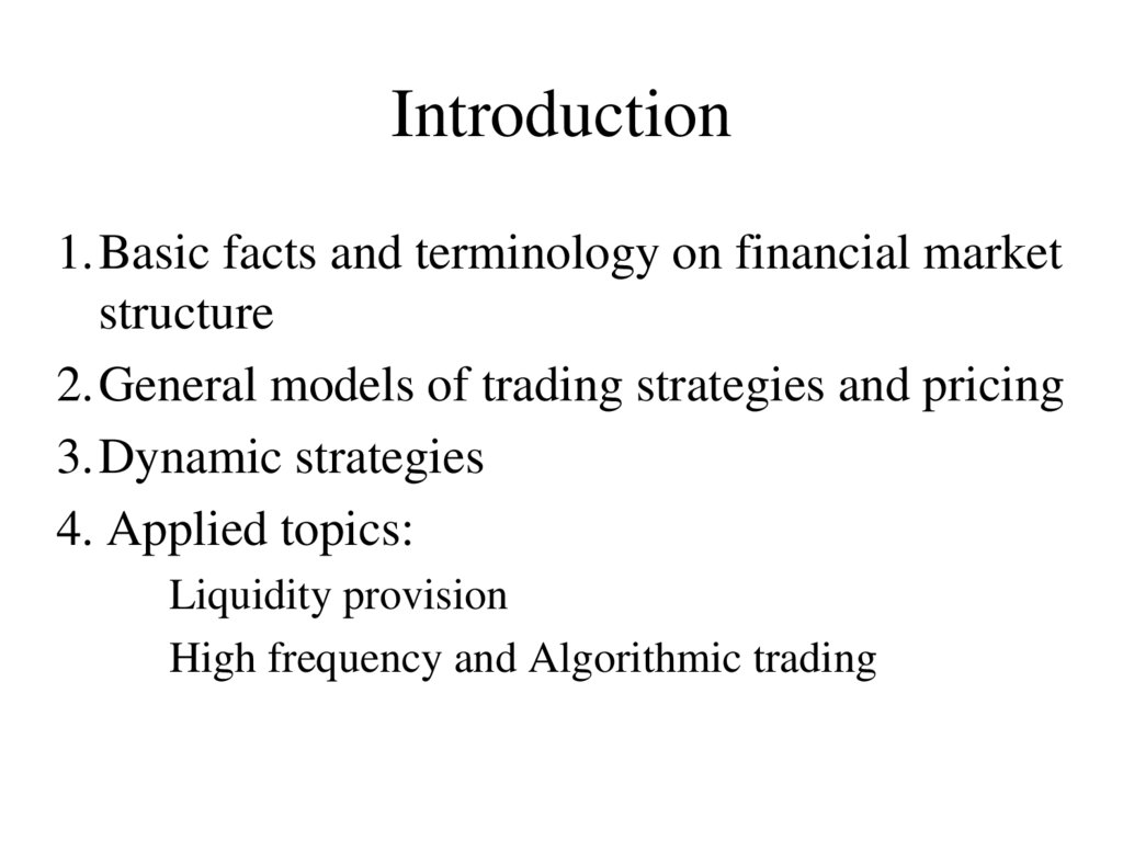
1.Basic facts and terminology on financial market
structure
2.General models of trading strategies and pricing
3.Dynamic strategies
4. Applied topics:
Liquidity provision
High frequency and Algorithmic trading

3. 1. Basic Facts and Terminology

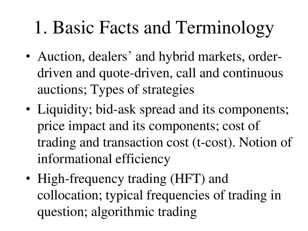
• Auction, dealers’ and hybrid markets, orderdriven and quote-driven, call and continuous
auctions; Types of strategies
• Liquidity; bid-ask spread and its components;
price impact and its components; cost of
trading and transaction cost (t-cost). Notion of
informational efficiency
• High-frequency trading (HFT) and
collocation; typical frequencies of trading in
question; algorithmic trading

4. Types of Markets

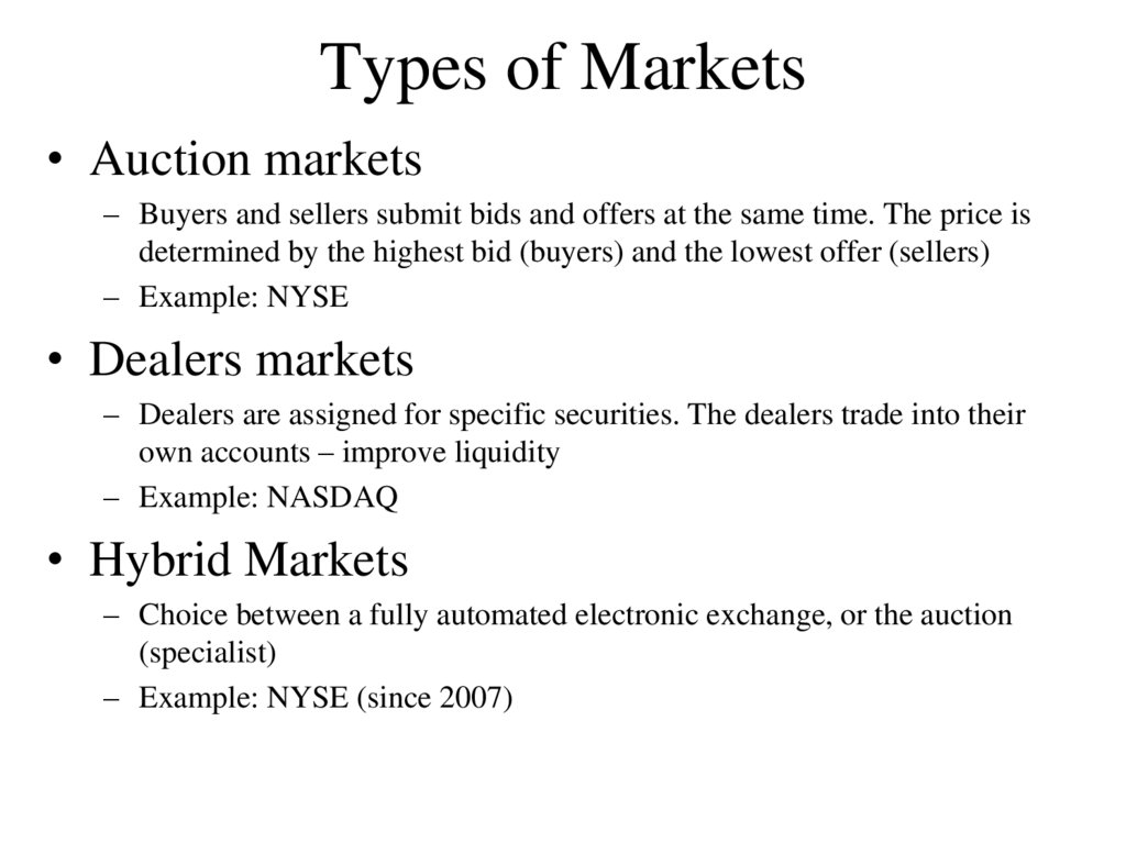
• Auction markets
– Buyers and sellers submit bids and offers at the same time. The price is
determined by the highest bid (buyers) and the lowest offer (sellers)
– Example: NYSE
• Dealers markets
– Dealers are assigned for specific securities. The dealers trade into their
own accounts – improve liquidity
– Example: NASDAQ
• Hybrid Markets
– Choice between a fully automated electronic exchange, or the auction
(specialist)
– Example: NYSE (since 2007)

5. Types of Markets (contd)

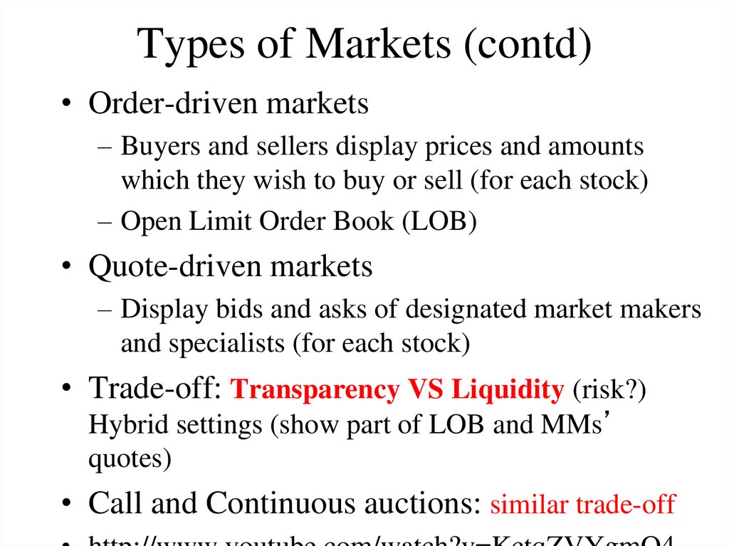
• Order-driven markets
– Buyers and sellers display prices and amounts
which they wish to buy or sell (for each stock)
– Open Limit Order Book (LOB)
• Quote-driven markets
– Display bids and asks of designated market makers
and specialists (for each stock)
• Trade-off: Transparency VS Liquidity (risk?)
Hybrid settings (show part of LOB and MMs’
quotes)
• Call and Continuous auctions: similar trade-off

6. Types of Strategies

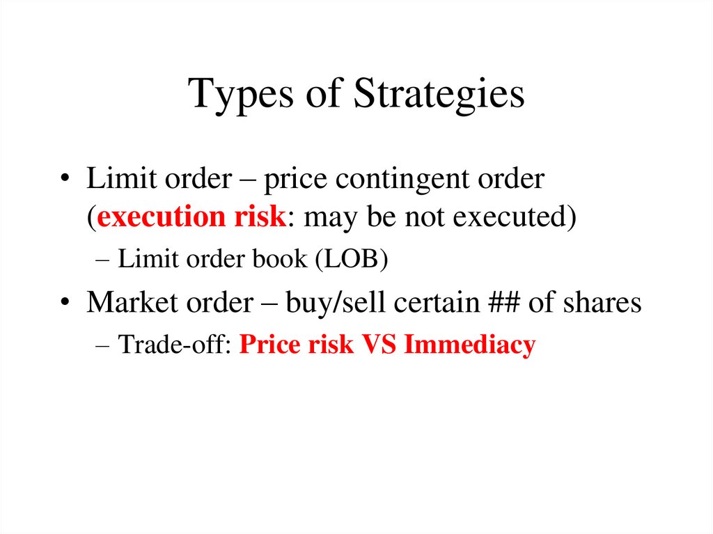
• Limit order – price contingent order
(execution risk: may be not executed)
– Limit order book (LOB)
• Market order – buy/sell certain ## of shares
– Trade-off: Price risk VS Immediacy

7. Types of Strategies (contd)

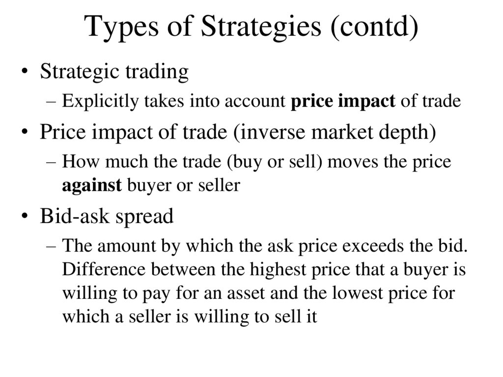
• Strategic trading
– Explicitly takes into account price impact of trade
• Price impact of trade (inverse market depth)
– How much the trade (buy or sell) moves the price
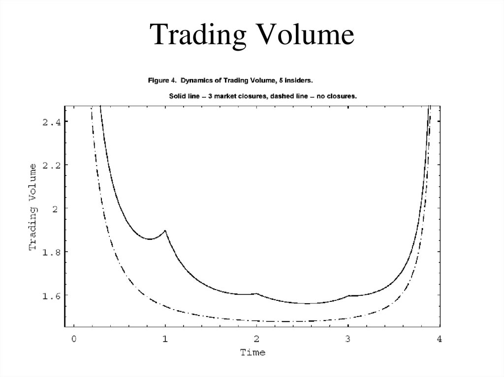
against buyer or seller
• Bid-ask spread
– The amount by which the ask price exceeds the bid.
Difference between the highest price that a buyer is
willing to pay for an asset and the lowest price for
which a seller is willing to sell it

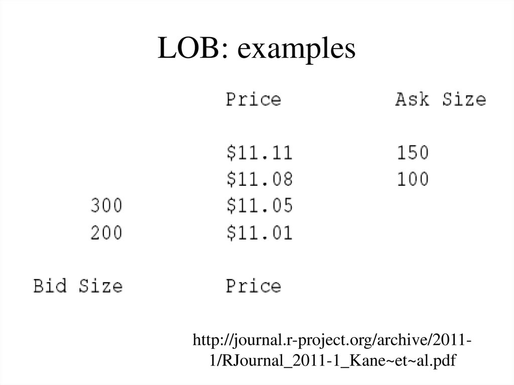
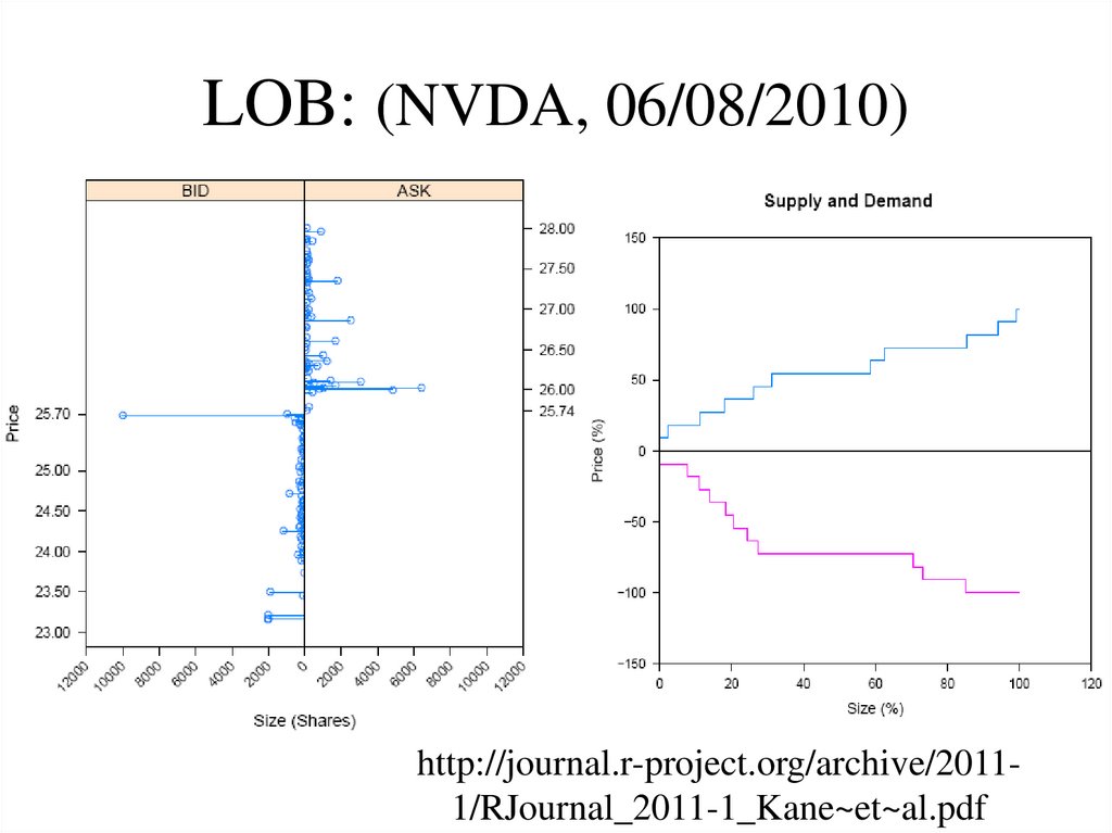
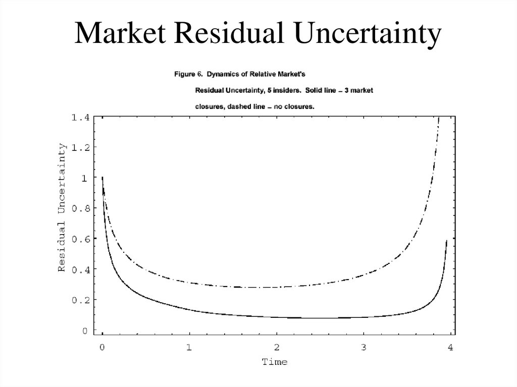
8. LOB: examples

http://journal.r-project.org/archive/20111/RJournal_2011-1_Kane~et~al.pdf

9. LOB: (NVDA, 06/08/2010)

http://journal.r-project.org/archive/20111/RJournal_2011-1_Kane~et~al.pdf

10. Market Liquidity and Efficiency: Multiple Dimension

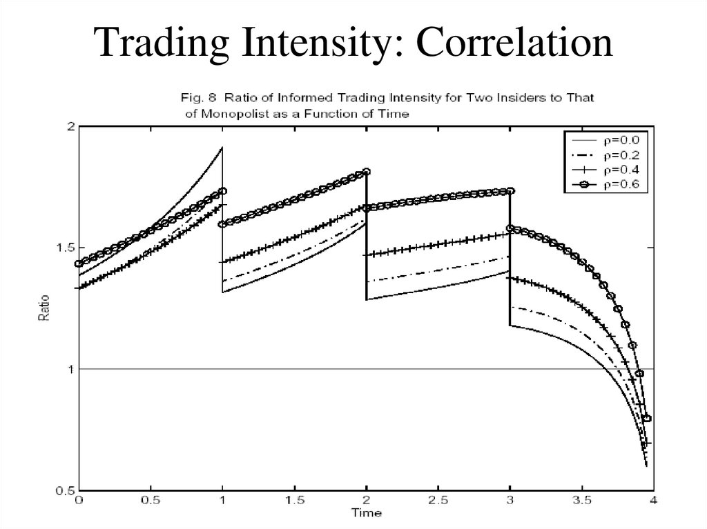
• Bid-ask spread
– Permanent (information-related) and temporary
(inventory) components
• Price impact
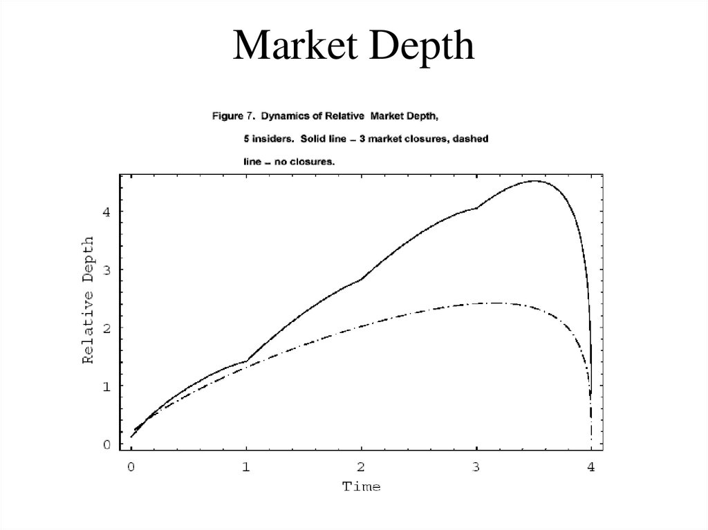
– Static and temporary components
• Cost of trading and transaction cost (t-cost)
– Price impact and fixed cost
• Informational efficiency
– Information content of price

11. Algorithmic and High Frequency Trading

• Algorithmic Trading and Optimal Execution
– Does not imply HF
– Objective: trade certain amount, minimize t-cost, risk
– Mean-variance approach (Almgren, Chriss)
– VWAP strategies (Volume Weighted Average Price)
Brokers try to buy below and then track VWAP
• High-frequency trading (HFT) and collocation
• Typical frequencies of trading in question
– Milliseconds (10^-3 s) (routing); microseconds (10^-6)
(waveguides, essentially compete with light speed)

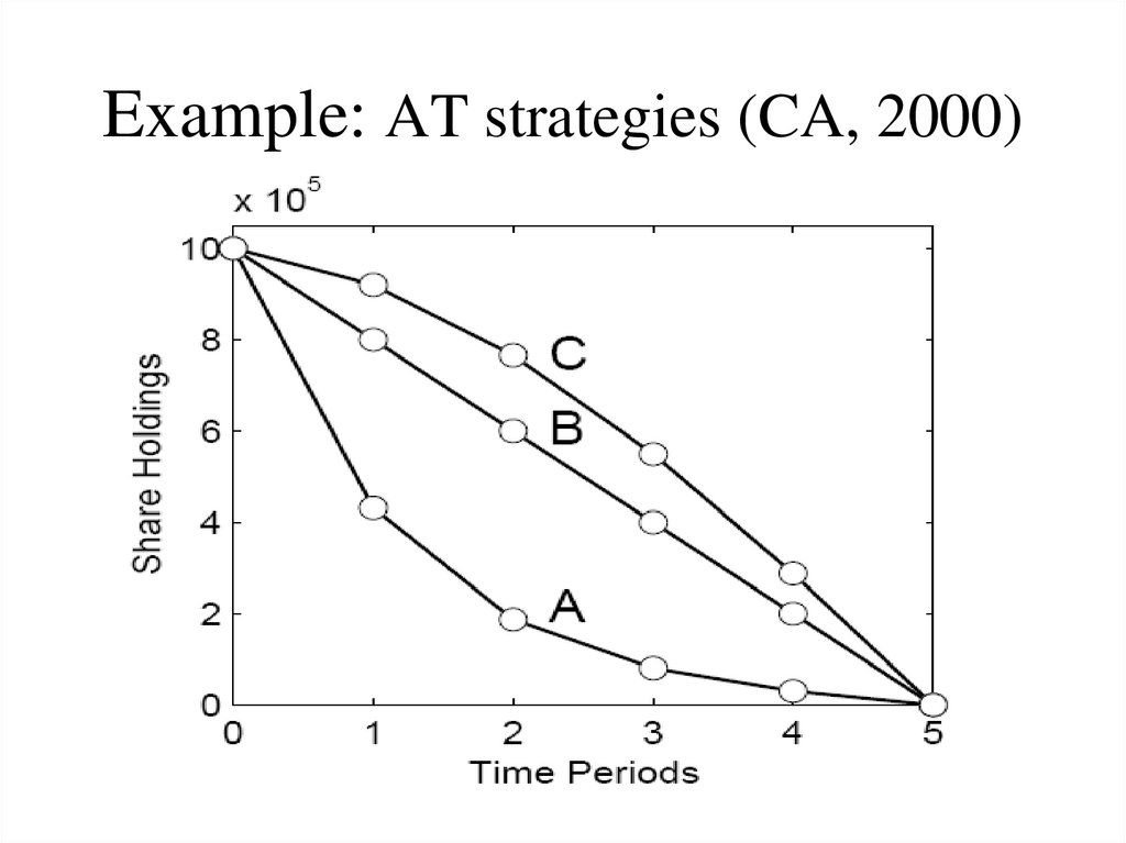
12. Example: AT strategies (CA, 2000)

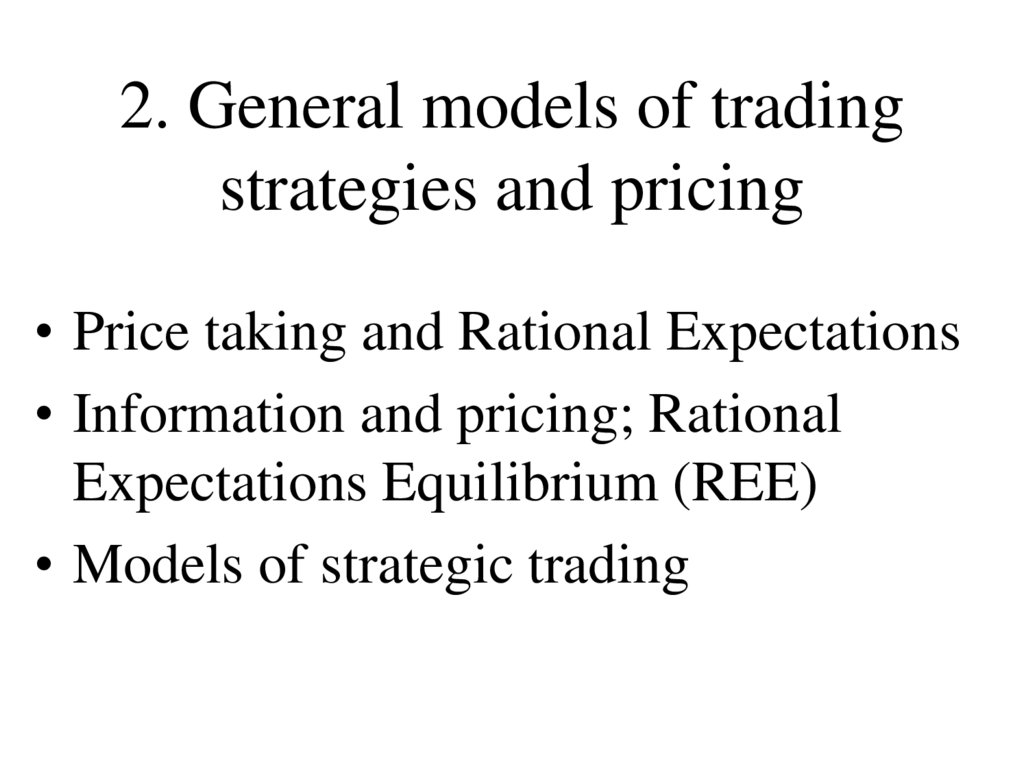
13. 2. General models of trading strategies and pricing

• Price taking and Rational Expectations
• Information and pricing; Rational
Expectations Equilibrium (REE)
• Models of strategic trading

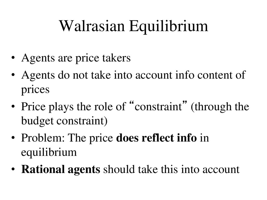
14. Walrasian Equilibrium

• Agents are price takers
• Agents do not take into account info content of
prices
• Price plays the role of “constraint” (through the
budget constraint)
• Problem: The price does reflect info in
equilibrium
• Rational agents should take this into account

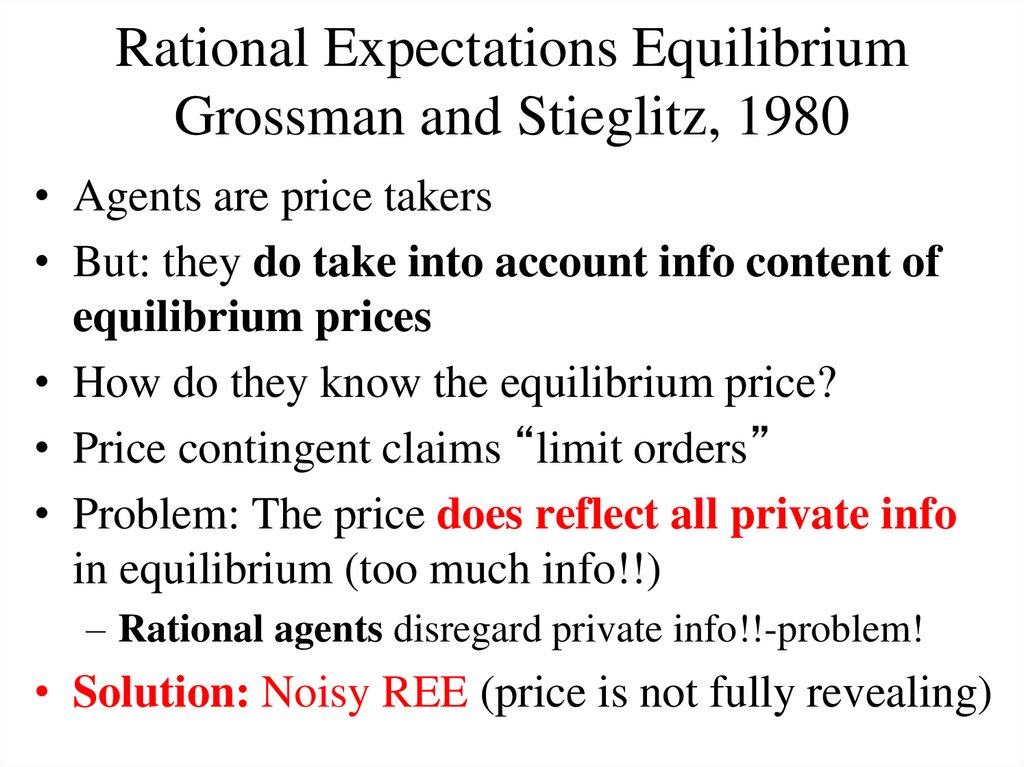
15. Rational Expectations Equilibrium Grossman and Stieglitz, 1980

• Agents are price takers
• But: they do take into account info content of
equilibrium prices
• How do they know the equilibrium price?
• Price contingent claims “limit orders”
• Problem: The price does reflect all private info
in equilibrium (too much info!!)
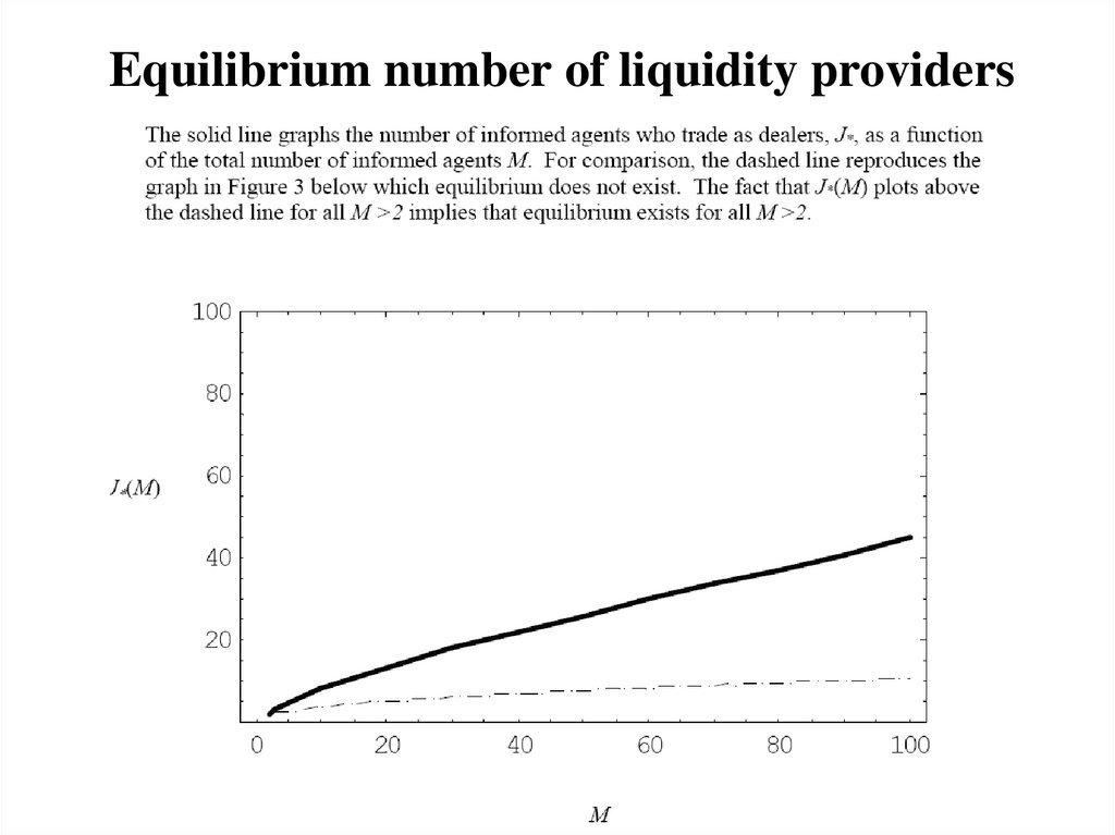
– Rational agents disregard private info!!-problem!
• Solution: Noisy REE (price is not fully revealing)

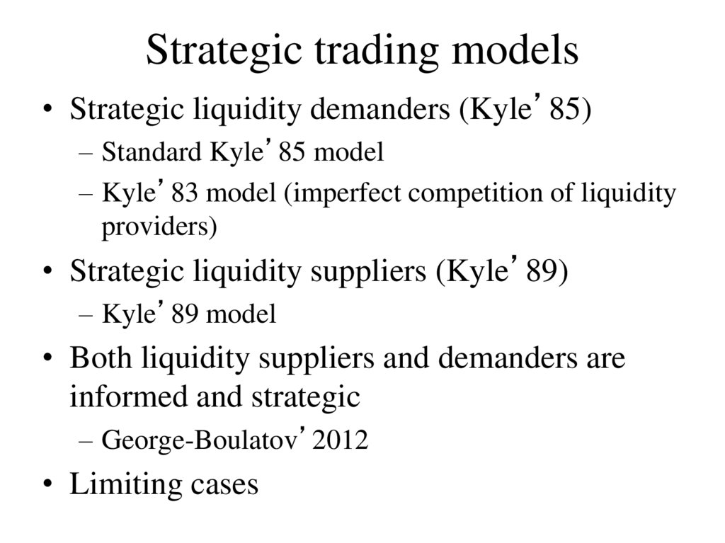
16. Strategic trading models

• Strategic liquidity demanders (Kyle’85)
– Standard Kyle’85 model
– Kyle’83 model (imperfect competition of liquidity
providers)
• Strategic liquidity suppliers (Kyle’89)
– Kyle’89 model
• Both liquidity suppliers and demanders are
informed and strategic
– George-Boulatov’2012
• Limiting cases

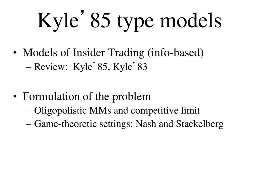
17. Kyle’85 type models

• Models of Insider Trading (info-based)
– Review: Kyle’85, Kyle’83
• Formulation of the problem
– Oligopolistic MMs and competitive limit
– Game-theoretic settings: Nash and Stackelberg

18. References

• Albert S. Kyle, 1985, “Continuous Auctions and Informed Trader
Trading”, Econometrica 53, 1315-1335.
• Jean-Charles Rochet, and Jean-Luc Vila, 1994, “Insider Trading
without Normality”, Review of Economic Studies 61, 131-152.
• Alex Boulatov and Thomas J. George, 2012, “Hidden and
Displayed Liquidity in Securities Markets with Informed Liquidity
Providers”, Review of Financial Studies, forthcoming.
Continuous time models:
• Kerry Back, 1992, “Insider Trading in Continuous Time”, The
Review of Financial Studies 5, 387-409.
Other related papers:
• Kyung-Ha Cho, and Nicole Karoui, 2000, “Insider Trading and
Nonlinear Equilibria: Single Auction Case”, Annales D’Economie
et de Statistique 60, 21-41.

19. Info-based models of insider trading

• Strategic nature of trading
• Motivation:
– Asset pricing models, (Back’92)

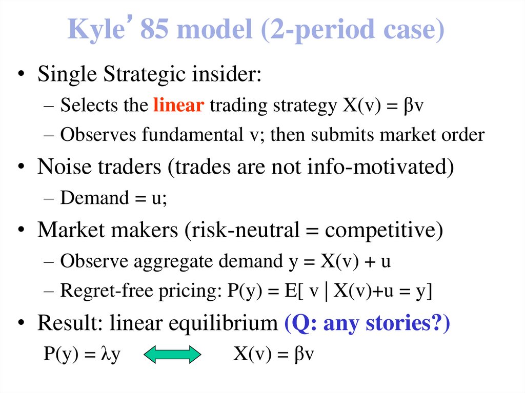
20. Kyle’85 model (2-period case)

• Single Strategic insider:
– Selects the linear trading strategy X(v) = βv
– Observes fundamental v; then submits market order
• Noise traders (trades are not info-motivated)
– Demand = u;
• Market makers (risk-neutral = competitive)
– Observe aggregate demand y = X(v) + u
– Regret-free pricing: P(y) = E[ v | X(v)+u = y]
• Result: linear equilibrium (Q: any stories?)
P(y) = λy
X(v) = βv

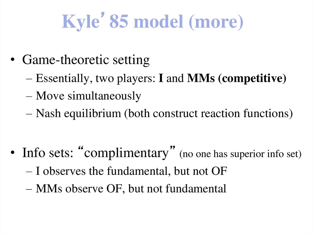
21. Kyle’85 model (more)

• Game-theoretic setting
– Essentially, two players: I and MMs (competitive)
– Move simultaneously
– Nash equilibrium (both construct reaction functions)
• Info sets: “complimentary” (no one has superior info set)
– I observes the fundamental, but not OF
– MMs observe OF, but not fundamental

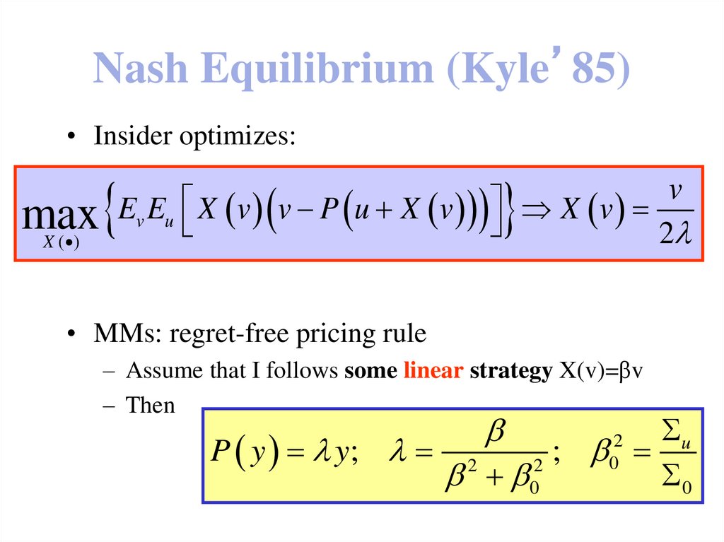
22. Nash Equilibrium (Kyle’85)

• Insider optimizes:
v
Ev Eu X v v P u X v X v
max
2
X ( )
• MMs: regret-free pricing rule
– Assume that I follows some linear strategy X(v)=βv
– Then
u
P y y; 2
;
2
0
0
2
0

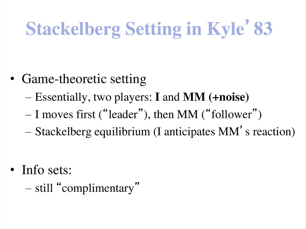
23. Stackelberg Setting in Kyle’83

• Game-theoretic setting
– Essentially, two players: I and MM (+noise)
– I moves first (“leader”), then MM (“follower”)
– Stackelberg equilibrium (I anticipates MM’s reaction)
• Info sets:
– still “complimentary”

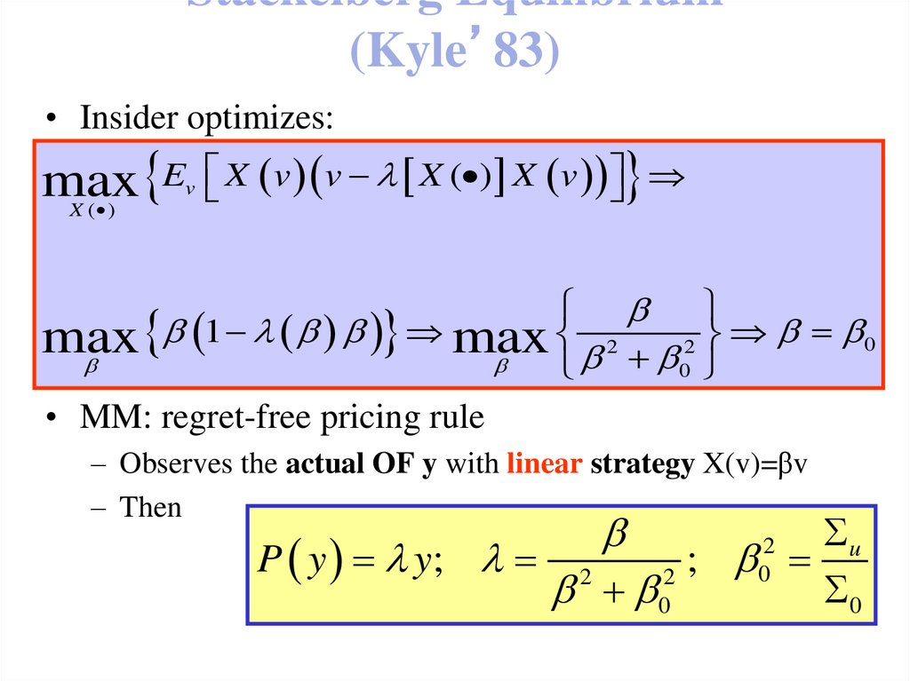
24. Stackelberg Equilibrium (Kyle’83)

• Insider optimizes:
max E X v v X ( ) X v
v
X ( )
1 max 2
0
max
2
0
• MM: regret-free pricing rule
– Observes the actual OF y with linear strategy X(v)=βv
– Then
u
P y y; 2
;
2
0
0
2
0

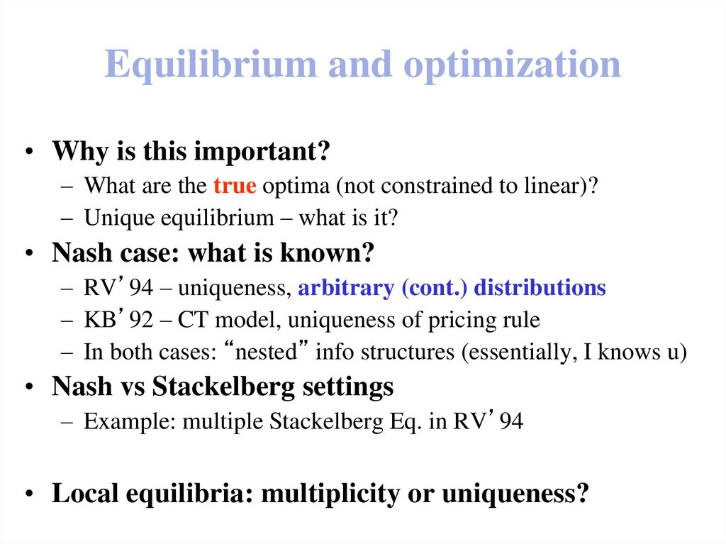
25. Equilibrium and optimization

• Why is this important?
– What are the true optima (not constrained to linear)?
– Unique equilibrium – what is it?
• Nash case: what is known?
– RV’94 – uniqueness, arbitrary (cont.) distributions
– KB’92 – CT model, uniqueness of pricing rule
– In both cases: “nested” info structures (essentially, I knows u)
• Nash vs Stackelberg settings
– Example: multiple Stackelberg Eq. in RV’94
• Local equilibria: multiplicity or uniqueness?

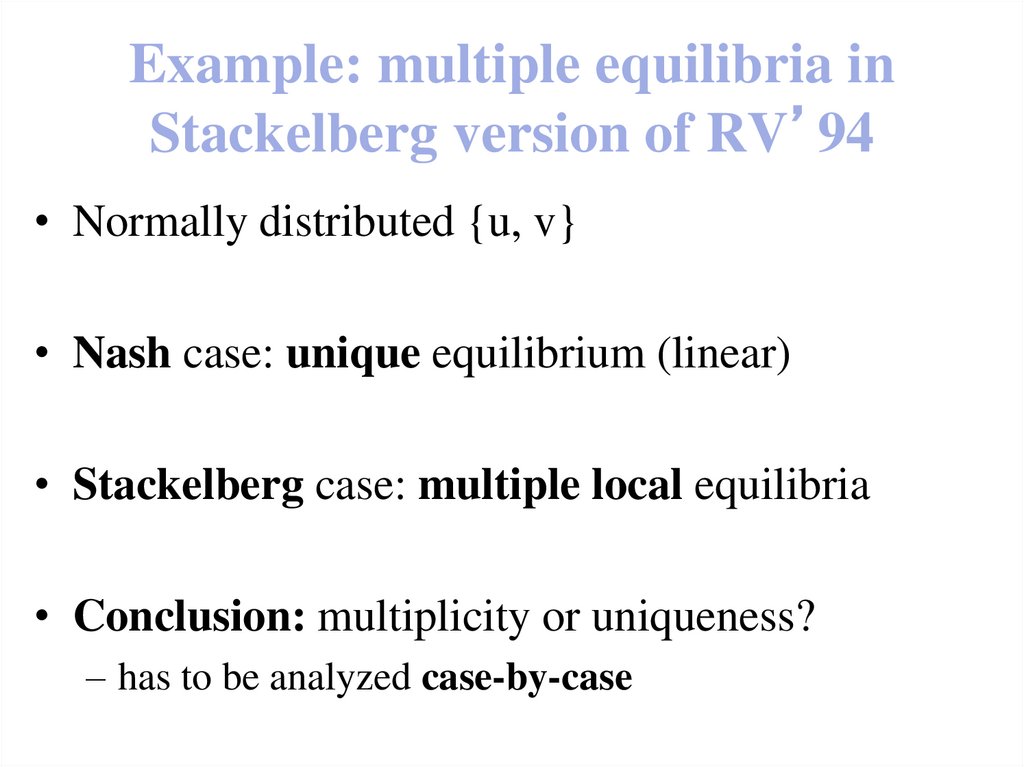
26. Example: multiple equilibria in Stackelberg version of RV’94

• Normally distributed {u, v}
• Nash case: unique equilibrium (linear)
• Stackelberg case: multiple local equilibria
• Conclusion: multiplicity or uniqueness?
– has to be analyzed case-by-case

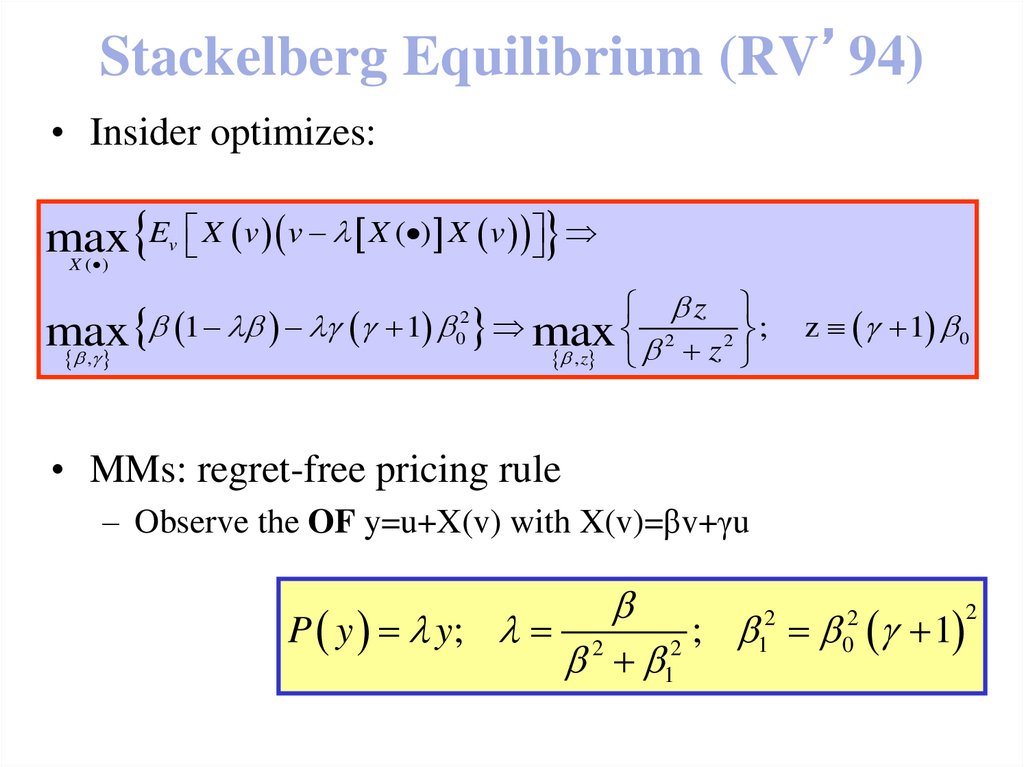
27. Stackelberg Equilibrium (RV’94)

• Insider optimizes:
max E X v v X ( ) X v
X ( )
v
z
1 1 max 2
;
max
2
,
, z z
2
0
z 1 0
• MMs: regret-free pricing rule
– Observe the OF y=u+X(v) with X(v)=βv+γu
P y y;
2
2
1
; 1
2
1
2
0
2

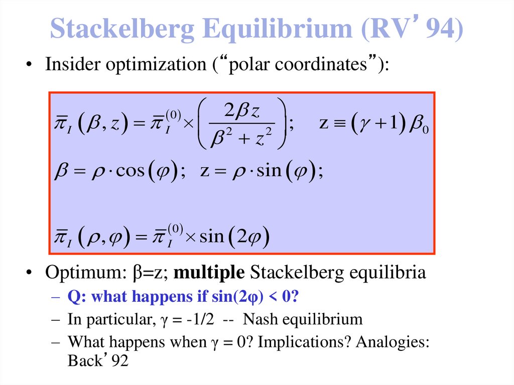
28. Stackelberg Equilibrium (RV’94)

• Insider optimization (“polar coordinates”):
2 z
I , z I 2
; z 1 0
2
z
cos ; z sin ;
0
I , I 0 sin 2
• Optimum: β=z; multiple Stackelberg equilibria
– Q: what happens if sin(2φ) < 0?
– In particular, γ = -1/2 -- Nash equilibrium
– What happens when γ = 0? Implications? Analogies:
Back’92

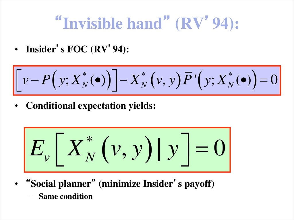
29. “Invisible hand” (RV’94):

• Insider’s FOC (RV’94):
v P y; X N* ( ) X N* v, y P ' y; X N* ( ) 0
• Conditional expectation yields:
Ev X
*
N
v, y | y 0
• “Social planner” (minimize Insider’s payoff)
– Same condition

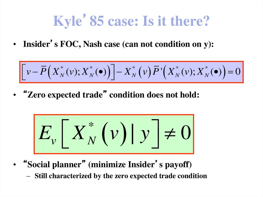
30. Kyle’85 case: Is it there?

• Insider’s FOC, Nash case (can not condition on y):
v P X N* (v); X N* ( ) X N* v P ' X N* (v); X N* ( ) 0
• “Zero expected trade” condition does not hold:
Ev X
*
N
v | y 0
• “Social planner” (minimize Insider’s payoff)
– Still characterized by the zero expected trade condition

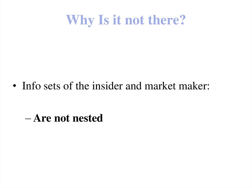
31. Why Is it not there?

• Info sets of the insider and market maker:
– Are not nested

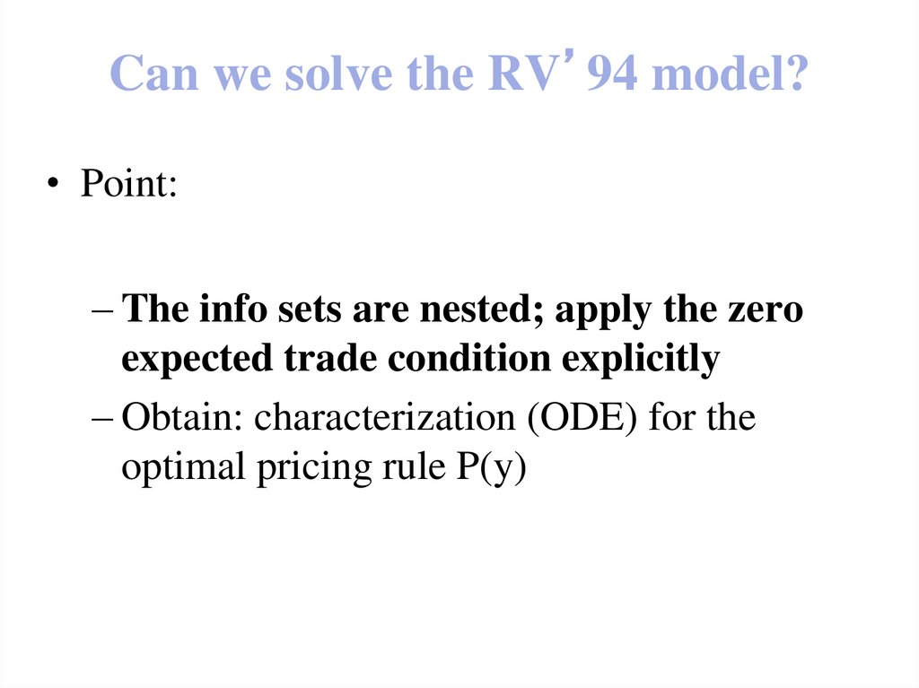
32. Can we solve the RV’94 model?

• Point:
– The info sets are nested; apply the zero
expected trade condition explicitly
– Obtain: characterization (ODE) for the
optimal pricing rule P(y)

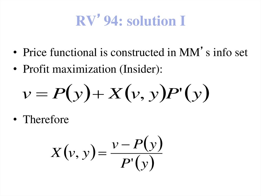
33. RV’94: solution I

• Price functional is constructed in MM’s info set
• Profit maximization (Insider):
v P y X v, y P' y
• Therefore
v P y
X v, y
P' y

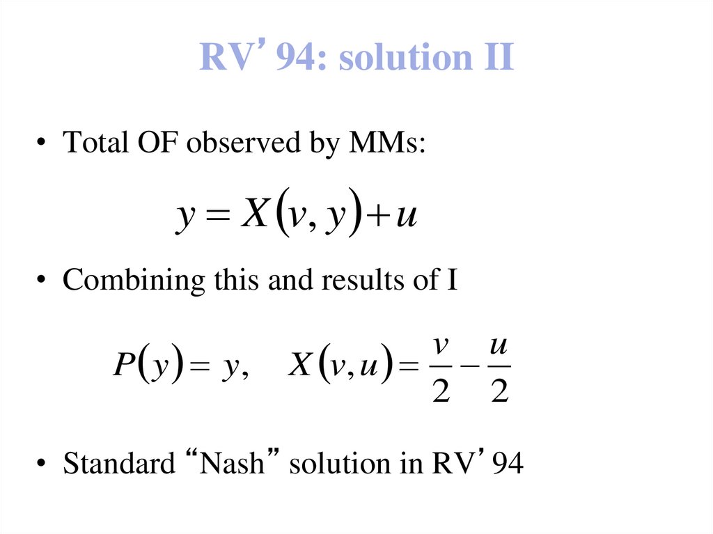
34. RV’94: solution II

• Total OF observed by MMs:
y X v, y u
• Combining this and results of I
P y y,
v u
X v, u
2 2
• Standard “Nash” solution in RV’94

35. Kyle’89 model

• Strategic informed liquidity suppliers
• Strategic uninformed liquidity suppliers
• Both types:
– Submit limit orders
– “Strategic limit order game”
• Liquidity (noise) traders
– Liquidity demanders (submit market orders)

36. 3. Dynamic strategies

• Dynamic trading strategies: discrete and
continuous time models
• Liquidity and algorithmic trading
• Optimal execution
• "Predatory trading" and "front running"

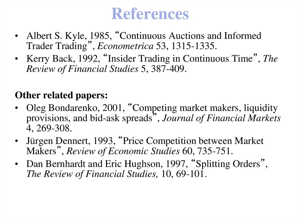
37. References

• Albert S. Kyle, 1985, “Continuous Auctions and Informed
Trader Trading”, Econometrica 53, 1315-1335.
• Kerry Back, 1992, “Insider Trading in Continuous Time”, The
Review of Financial Studies 5, 387-409.
Other related papers:
• Oleg Bondarenko, 2001, “Competing market makers, liquidity
provisions, and bid-ask spreads”, Journal of Financial Markets
4, 269-308.
• Jürgen Dennert, 1993, “Price Competition between Market
Makers”, Review of Economic Studies 60, 735-751.
• Dan Bernhardt and Eric Hughson, 1997, “Splitting Orders”,
The Review of Financial Studies, 10, 69-101.

38. Outline

• Dynamic Models of Informed Trading
– Review: Kyle’85
• Dynamic Bayesian Equilibria: typical features
– Review: Kyle’85, Back’92, Bondarenko’ 2001
• Formulation of the problem
– Game-theoretic settings: Dynamic Bayesian Nash
– Reduction to one- or two-sided optimization
• Solutions: an overview

39. Dynamic Informed Trading

• Why is this important?
– One of the fundamental issues of the MS theory
– Kyle [1985]: an example of CT insider trading
• Features:
– Constant market depth over time
– Private info is totally reflected in price at t = T
• Extensions:
– Relax the ME assumption: Dealers make money
– Inter-dealer competition: Informed dealers

40. Insider trading and liquidity provision

• Strategic nature of insider trading
• Lifting the market efficiency condition:
– Dealers are making profits (imperfect
competition)
• two-sided strategic trading (Dennert’93)

41. Kyle’85 model: CT setting

• Game-theoretic setting
– Essentially, two types players: I and MMs (+noise)
• Info sets:
– still “complimentary”
• Multiple auctions

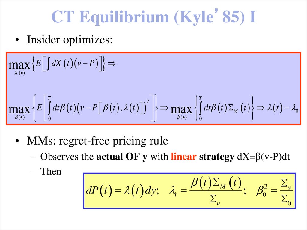
42. CT Equilibrium (Kyle’85) I

• Insider optimizes:
max E dX t v P
X ( )
T
2
T
E dt t v P t , t max dt t M t t 0
max
( )
( ) 0
0
• MMs: regret-free pricing rule
– Observes the actual OF y with linear strategy dX=β(v-P)dt
– Then
dP t t dy; t
t M t
u
u
;
0
2
0

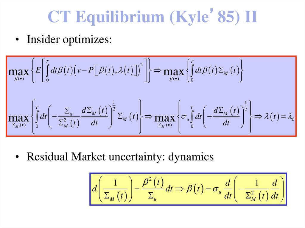
43. CT Equilibrium (Kyle’85) II

• Insider optimizes:
T
2
T
E dt t v P t , t max dt t M t
max
( )
( ) 0
0
1
1
T
T
2
2
d
t
d
t
u
M
M
dt
t
dt
max u
t 0
M
max
2
dt
M ( ) 0
M ( )
0
M t dt
• Residual Market uncertainty: dynamics
1 2 t
d
1 d
d
dt t u 2
u
dt M t dt
M t

44. Resulting equilibrium

• Why is this important?
– Dynamic trading strategies – more realistic
– Global optimization (insider’s problem)
• Stackelberg case: is it different?
– In both cases: same answer (different methodology)
• Other equilibria: Nash vs Stackelberg cases
– Example: multiple static Stackelberg Eq. in RV’94
• Dynamic equilibria: multiplicity or uniqueness?

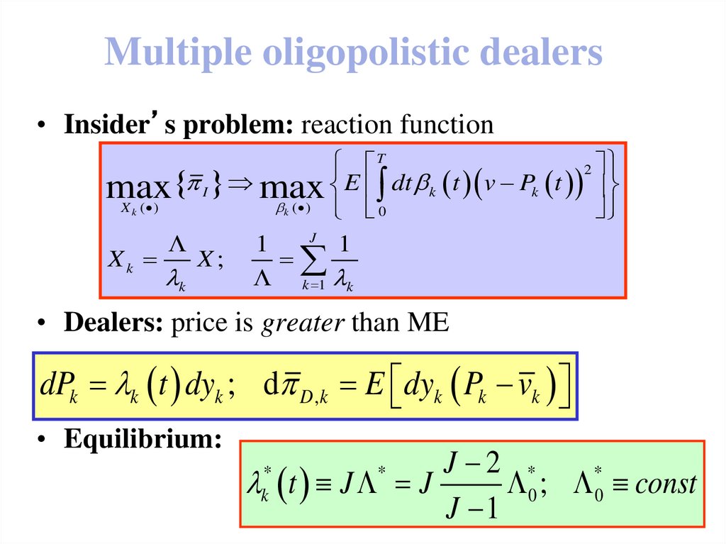
45. Multiple oligopolistic dealers

• Insider’s problem: reaction function
T
2
I max E dt k t v Pk t
max
X k ( )
k ( )
0
J
1
1
Xk
X;
k
k 1 k
• Dealers: price is greater than ME
dPk k t dyk ; d D ,k E dyk Pk vk
• Equilibrium:
J 2 *
*
t J J
0 ; 0 const
J 1
*
k
*

46. Conclusions

• Dynamic CT linear equilibrium from Kyle’85
– Same in Nash and Stackelberg cases
• The CT version of Bondarenko’01

47. Dynamic Private Information: Multiple Signals

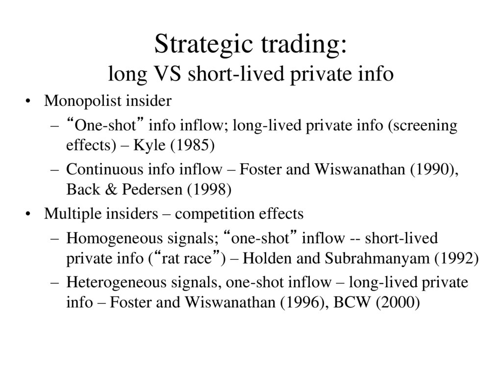
Boulatov and Livdan, 2011

48. Strategic trading: long VS short-lived private info

• Monopolist insider
– “One-shot” info inflow; long-lived private info (screening
effects) – Kyle (1985)
– Continuous info inflow – Foster and Wiswanathan (1990),
Back & Pedersen (1998)
• Multiple insiders – competition effects
– Homogeneous signals; “one-shot” inflow -- short-lived
private info (“rat race”) – Holden and Subrahmanyam (1992)
– Heterogeneous signals, one-shot inflow – long-lived private
info – Foster and Wiswanathan (1996), BCW (2000)

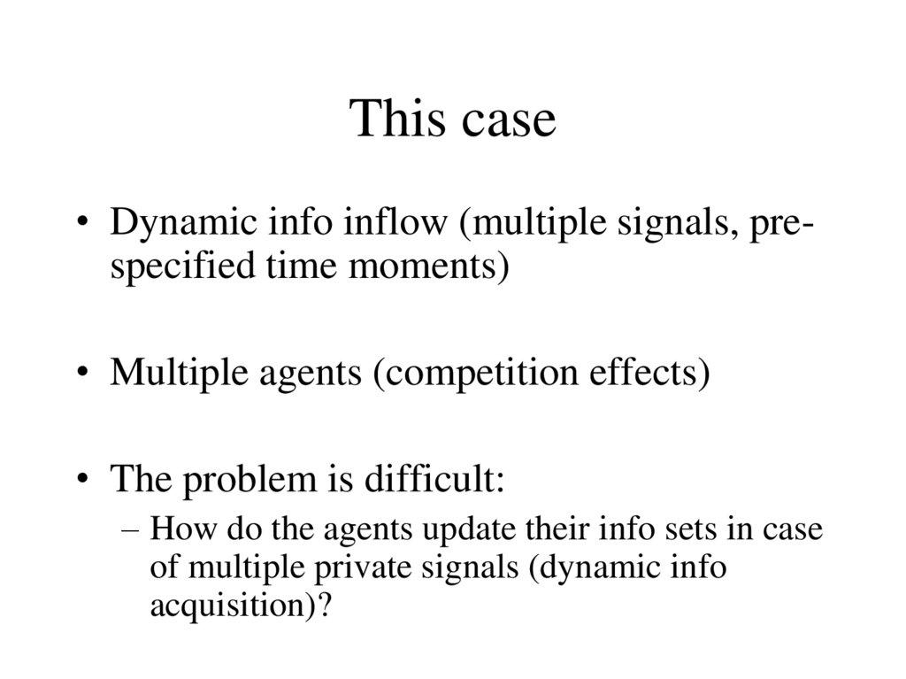
49. This case

• Dynamic info inflow (multiple signals, prespecified time moments)
• Multiple agents (competition effects)
• The problem is difficult:
– How do the agents update their info sets in case
of multiple private signals (dynamic info
acquisition)?

50. Our approach

• Focus on the dynamic info acquisition problem
• Use the existing dynamic “one-shot info” model
(BCW, 2000) as a “benchmark” -- analyze the
specific effect of dynamic info acquisition
• Discrete (private) info inflow
• Timing of new info arrival is public knowledge –
traders receive private signals when market is closed
– Motivation: info asymmetry increases when the market is
closed – French and Roll (1986), Ito, Lyons and Melvin
(1998)
– Empirical implications: U-shaped trading volume, nonperiodic structure

51. Long-horizon effects of MM: Info Story

• How is the arriving (dynamic) private info
incorporated in the market?
– multiple agents (Oligopoly)
– asymmetric information (heterogeneous signals)
– Information inflow (periodic)

52. Setting

• Oligopoly:
– agents have “complimentary” pieces of info,
i.e. aggregate signal is superior to any
individual one
• Therefore:
– agents learn both from Price (set by the MM
based on aggregate signal), and from private
signals

53. Static VS Dynamic Info

• Static Info
– Info distribution across agents:
• Perfectly correlated signals – “rat race”, no long-lived private
info
• Less than perfect correlation – “waiting phase” (screening),
private info is long-lived
• Dynamic Info
– Timing of Info (new “dimension”):
• Generally leads to more trading if the new info arrival is
anticipated (less incentive to screen the “old” info)

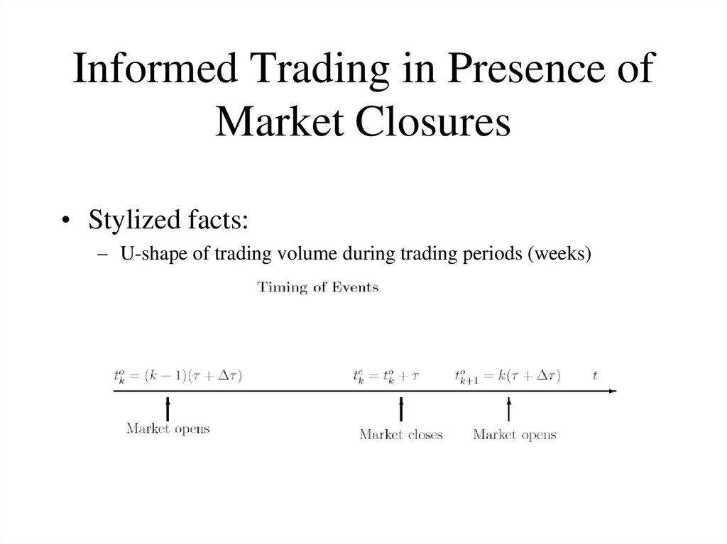
54. Informed Trading in Presence of Market Closures

• Stylized facts:
– U-shape of trading volume during trading periods (weeks)
– A-periodic temporal structure on larger time scales (months)

55. Comparison to the Existing Literature

• Holden & Subrahmanyam [1992]
– Perfectly correlated signals
– short-lived private info (as opposed to our case)
• Foster & Wishwanathan [1990, 1996]
– monopolist economy - additional assumptions to generate
trading patterns (announcements each period)
– non-strategic between different periods
• Hong & Wang [2000]
– periodic closures - symmetric equilibrium (periodic trading
patterns) - counterfactual

56. The Model I

• Agents:
The Model I
– N Insiders (I-informed traders): receive
noisy (heterogeneous) private signals; Learn
(price & signals)
– Market Maker (MM): observes aggregate
demand, sets regret-free price; Learns
(aggregate demand)
– Liquidity (noise) traders: sufficient #
• Market Closure periods: MM does not
learn, I keeps learning

57. The Model II

• Multi-period economy:
– 3 types of agents, 1 risky asset
– (analogous to Kyle [1985]; Back et al [2000])
• Risky asset:
– dividend (fundamental V) announced at
terminal date T

58. Sequence of Events

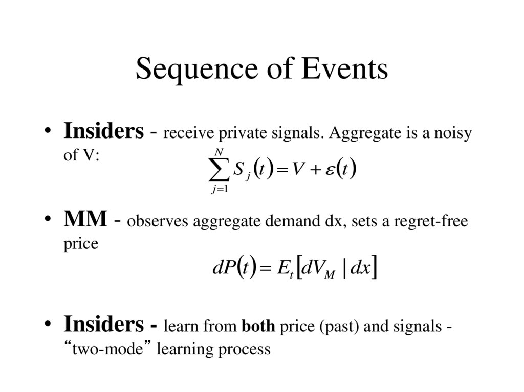
• Insiders - receive private signals. Aggregate is a noisy
of V:
N
S t V t
j 1
j
• MM - observes aggregate demand dx, sets a regret-free
price
dP t Et dVM | dx
• Insiders - learn from both price (past) and signals “two-mode” learning process

59. Equilibrium Strategies

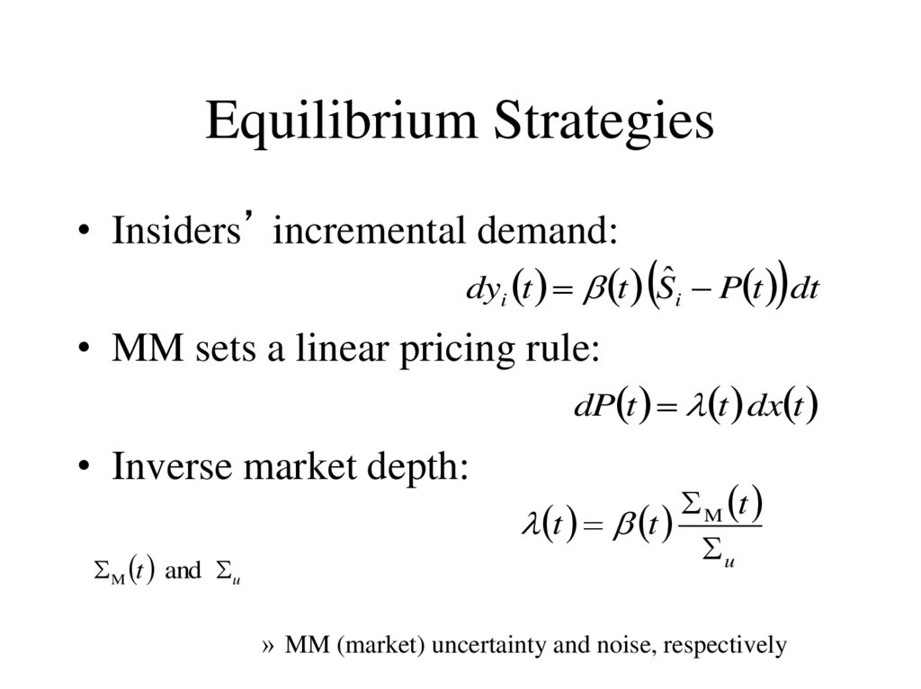
• Insiders’ incremental demand:
dyi t t Sˆi P t dt
• MM sets a linear pricing rule:
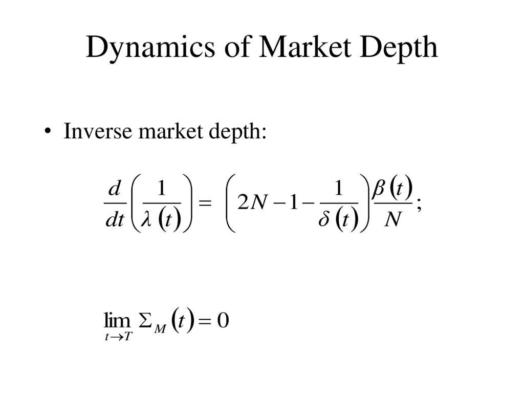
dP t t dx t
• Inverse market depth:
M t and u
M t
t t
u
» MM (market) uncertainty and noise, respectively

60. Learning I

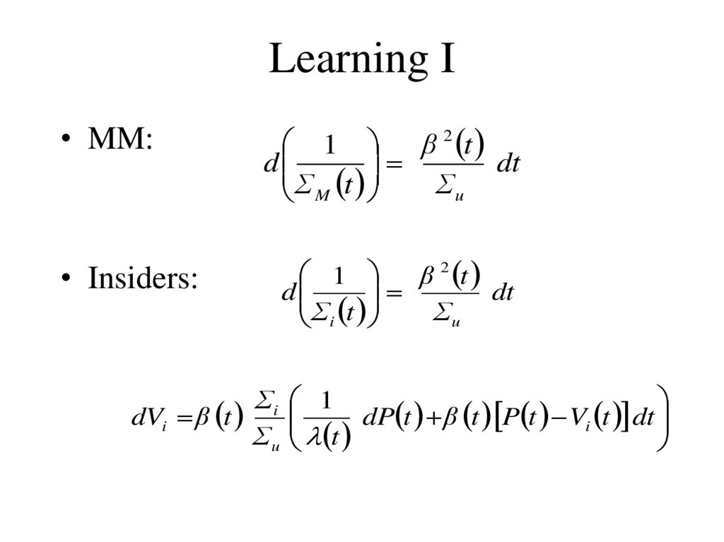
• MM:
1 β 2 t
d
dt
Σu
Σ M t
• Insiders:
1
β 2 t
d
dt
Σu
Σi t
Σi 1
dVi β t
dP t β t P t Vi t dt
Σ u t

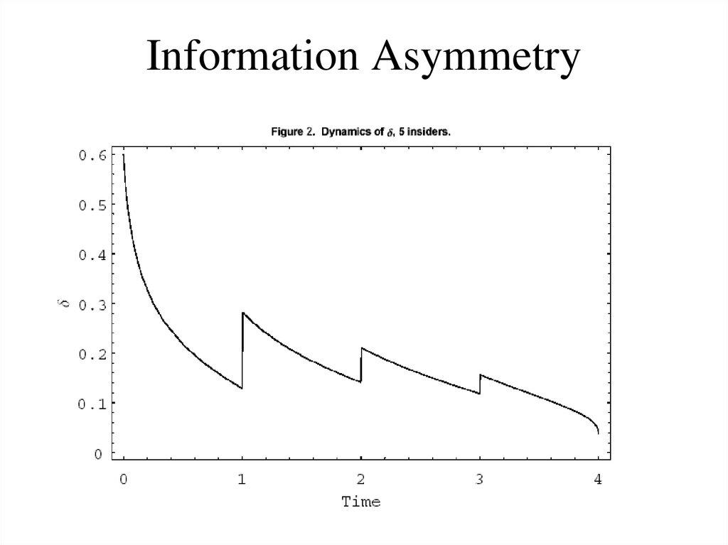
61. Learning II

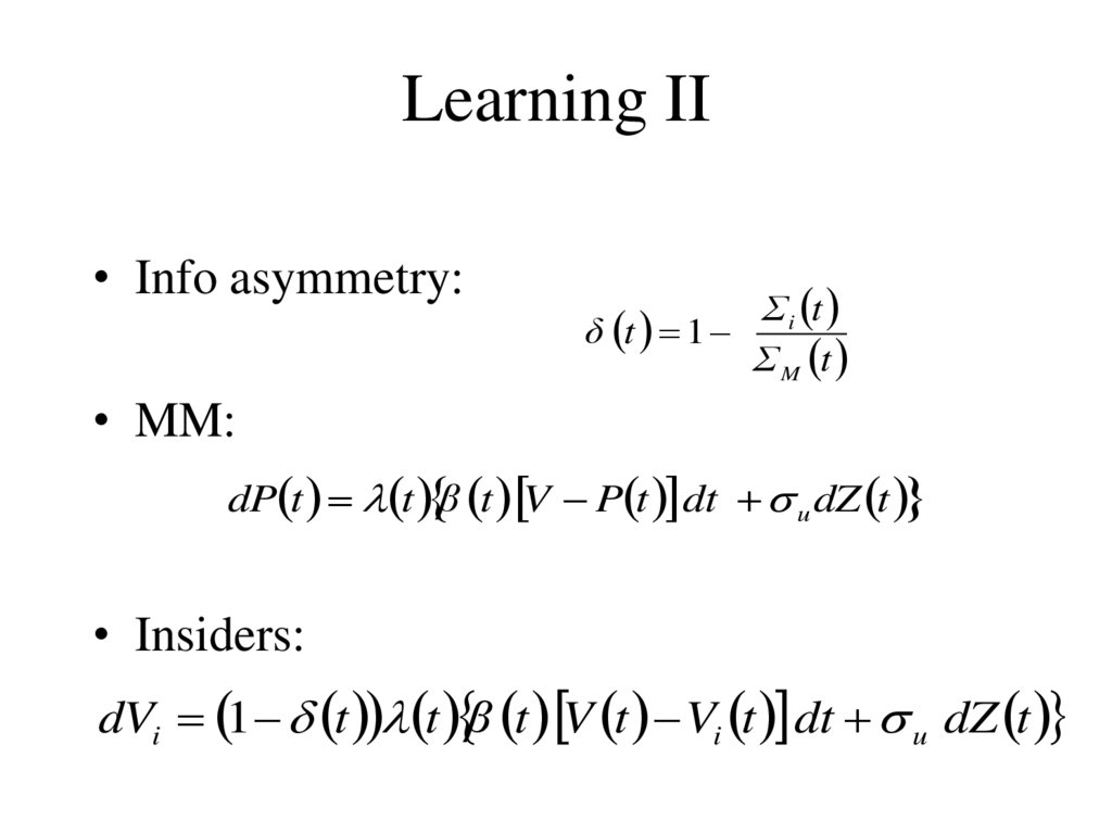
• Info asymmetry:
Σ i t
δ t 1
Σ M t
• MM:
dP t t β t V P t dt u dZ t
• Insiders:
dVi 1 t t β t V t Vi t dt u dZ t

62. Dynamic Trading Game

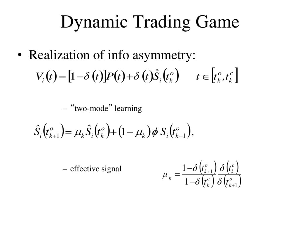
• Realization of info asymmetry:
Vi t 1 δ t P t δ t Sˆi tko
t tko ,tkc
– “two-mode” learning
Sˆi tko 1 k Sˆi tko 1 k Si tko 1 ,
– effective signal
1 δ t ko 1 δ t kc
μk
1 δ t kc δ t ko 1

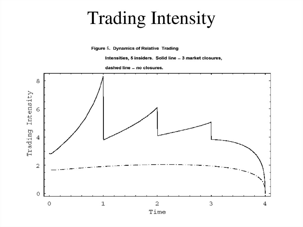
63. Implications for Trading Strategies

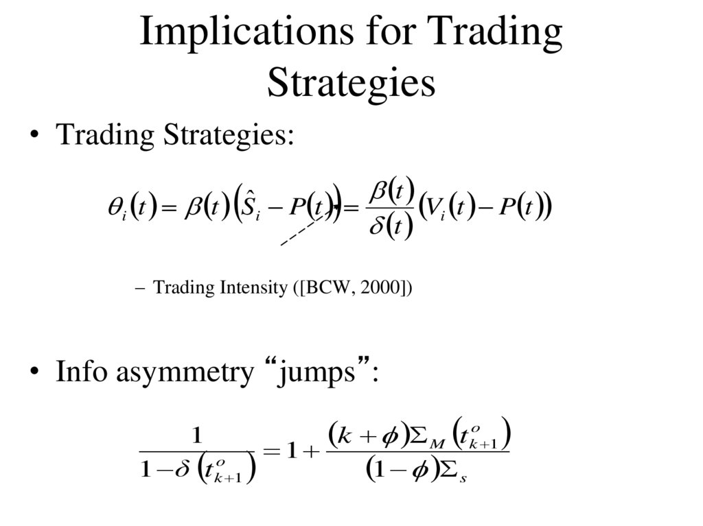
• Trading Strategies:
t
ˆ
Vi t P t
i t t Si P t
t
– Trading Intensity ([BCW, 2000])
• Info asymmetry “jumps”:
k M t ko 1
1
1
o
1 s
1 δ t k 1

64. Implications for Trading Volume

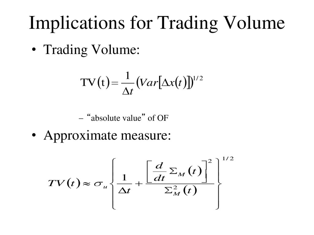
• Trading Volume:
1
Var x t 1/ 2
TV t
t
– “absolute value” of OF
• Approximate measure:
d
t
M
1
dt
TV t u
2
t
M t
2
1/ 2

65. Solution

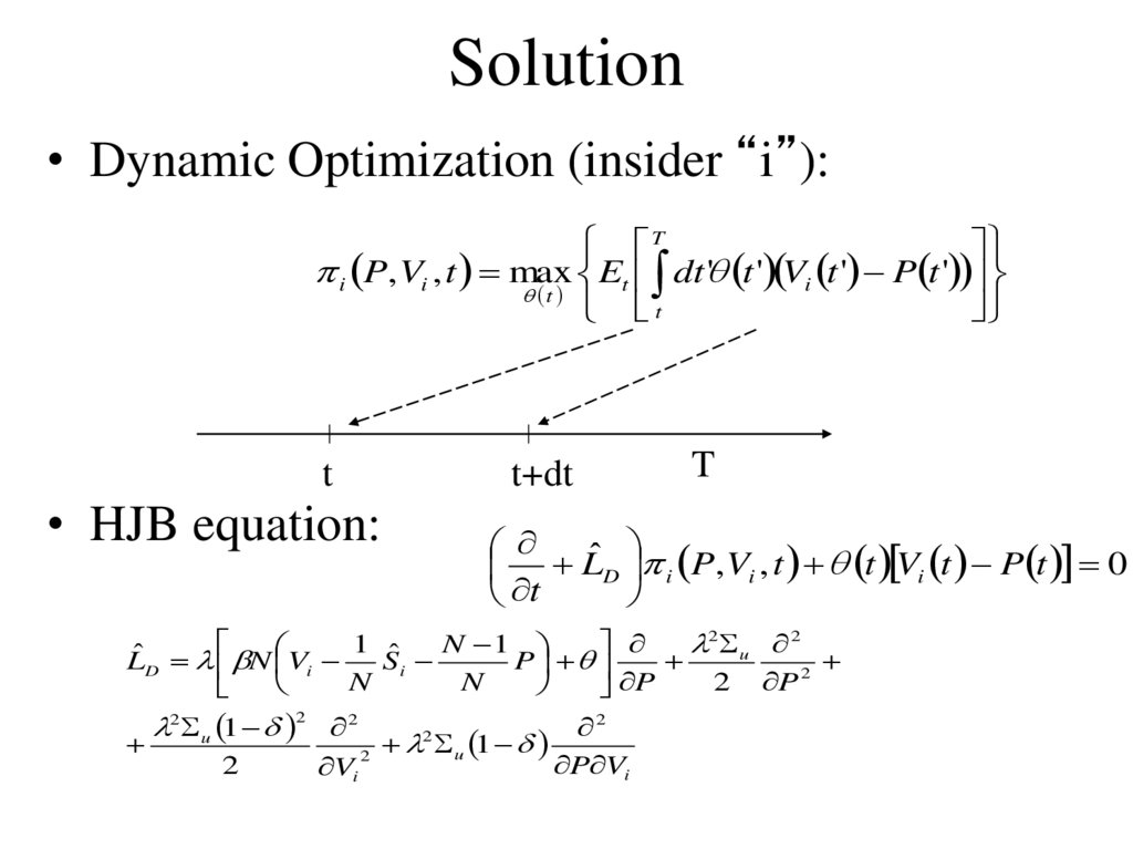
• Dynamic Optimization (insider “i”):
T
i P, Vi , t max Et dt
' t ' Vi t ' P t '
t
t
t
t+dt
• HJB equation:
T
Lˆ D i P, Vi , t t Vi t P t 0
t
2
2
1
N
1
u
Lˆ D N Vi
Sˆi
P
2
N
N
P
2
P
2 u 1 2 2
2
2
u 1
2
P Vi
Vi
2

66. Dynamics of Market Depth

• Inverse market depth:
d 1
1 β t
2 N 1
;
dt λ t
δ t N
lim M t 0
t T

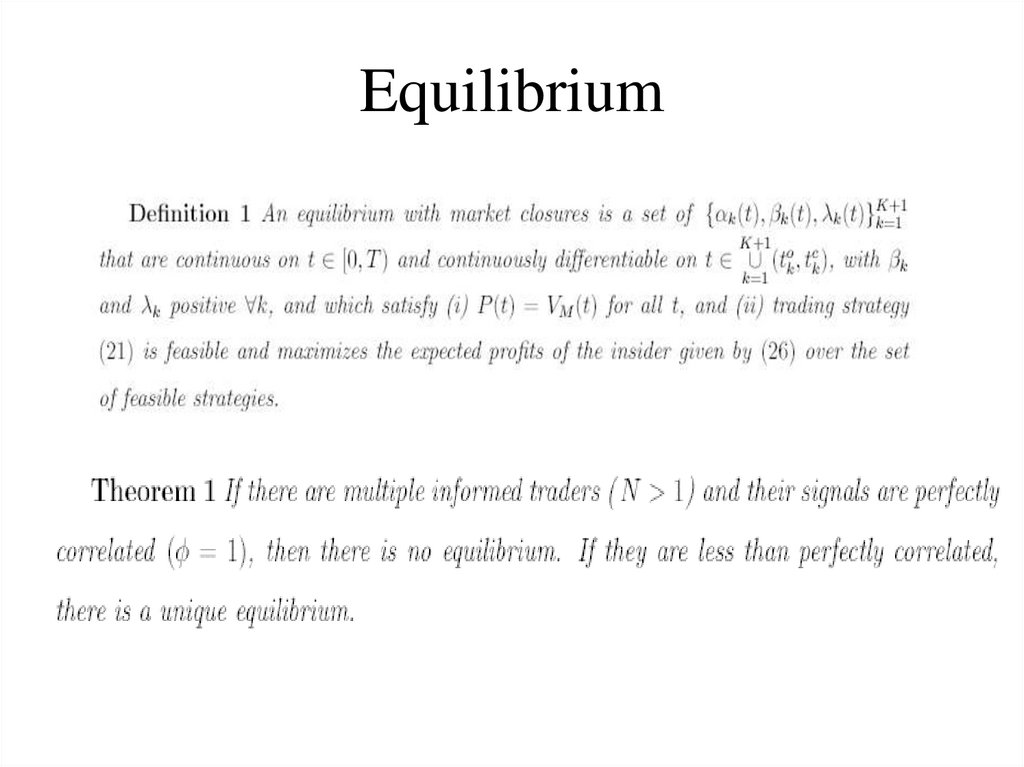
67. Equilibrium

68. Information Asymmetry

69. Trading Intensity

70. Trading Intensity: Correlation

71. Trading Volume

72. Market Residual Uncertainty

73. Market Depth

74. Conclusions

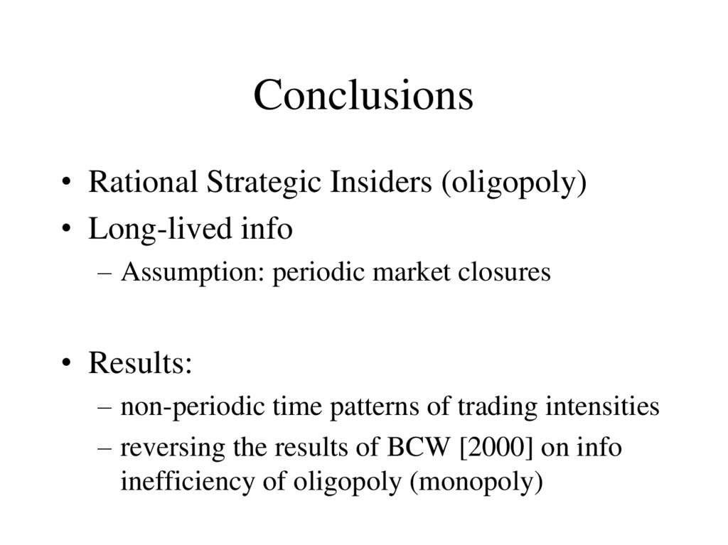
• Rational Strategic Insiders (oligopoly)
• Long-lived info
– Assumption: periodic market closures
• Results:
– non-periodic time patterns of trading intensities
– reversing the results of BCW [2000] on info
inefficiency of oligopoly (monopoly)

75. 4. Applied topics

• High-frequency and algorithmic trading
• Quality of markets and informed liquidity
provision
• Optimization of limited information resources
(limited attention).

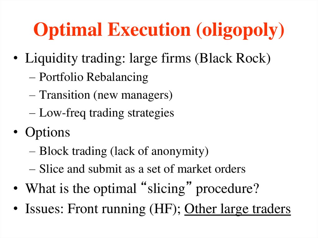
76. Optimal Execution (oligopoly)

• Liquidity trading: large firms (Black Rock)
– Portfolio Rebalancing
– Transition (new managers)
– Low-freq trading strategies
• Options
– Block trading (lack of anonymity)
– Slice and submit as a set of market orders
• What is the optimal “slicing” procedure?
• Issues: Front running (HF); Other large traders

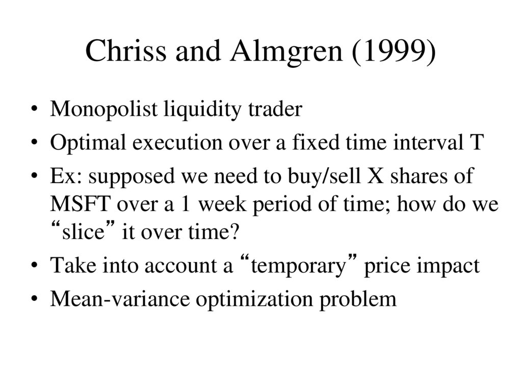
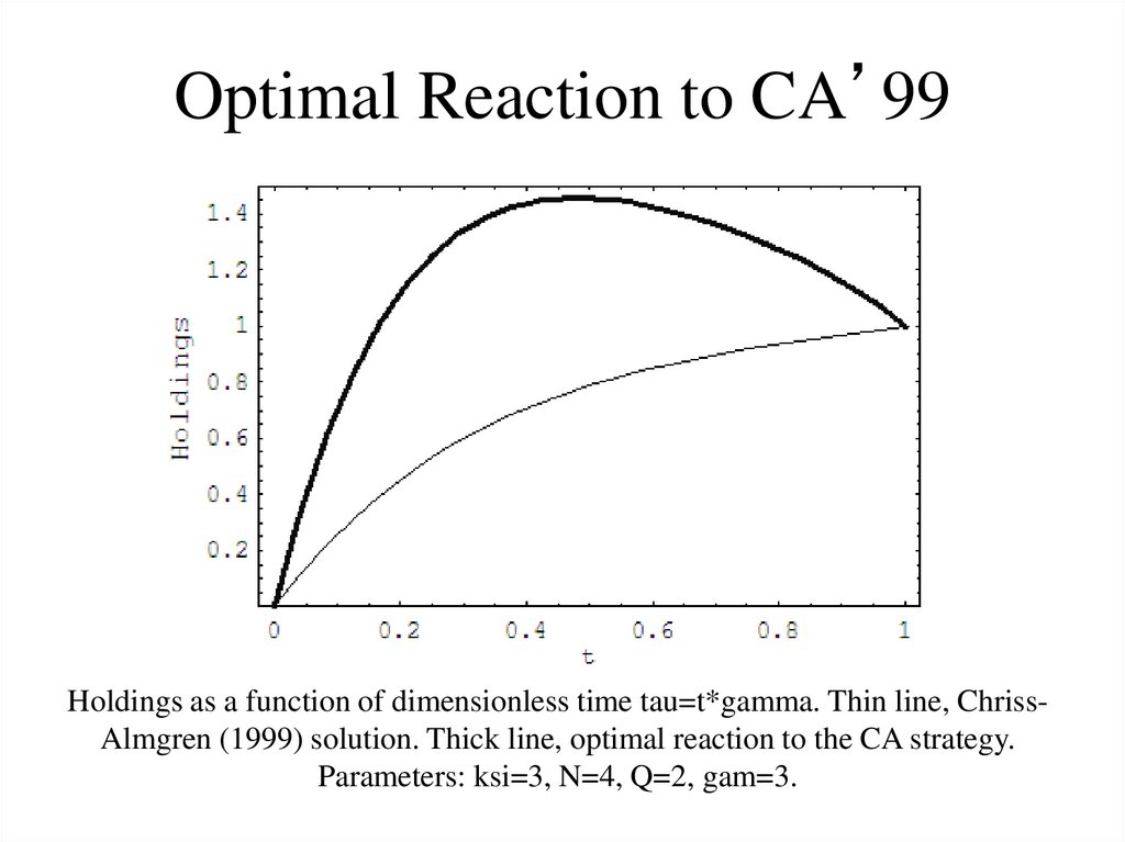
77. Chriss and Almgren (1999)

• Monopolist liquidity trader
• Optimal execution over a fixed time interval T
• Ex: supposed we need to buy/sell X shares of
MSFT over a 1 week period of time; how do we
“slice” it over time?
• Take into account a “temporary” price impact
• Mean-variance optimization problem

78. Optimal Reaction to CA’99

Holdings as a function of dimensionless time tau=t*gamma. Thin line, ChrissAlmgren (1999) solution. Thick line, optimal reaction to the CA strategy.
Parameters: ksi=3, N=4, Q=2, gam=3.

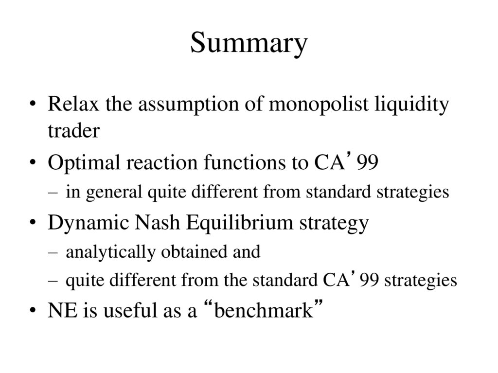
79. Summary

• Relax the assumption of monopolist liquidity
trader
• Optimal reaction functions to CA’99
– in general quite different from standard strategies
• Dynamic Nash Equilibrium strategy
– analytically obtained and
– quite different from the standard CA’99 strategies
• NE is useful as a “benchmark”

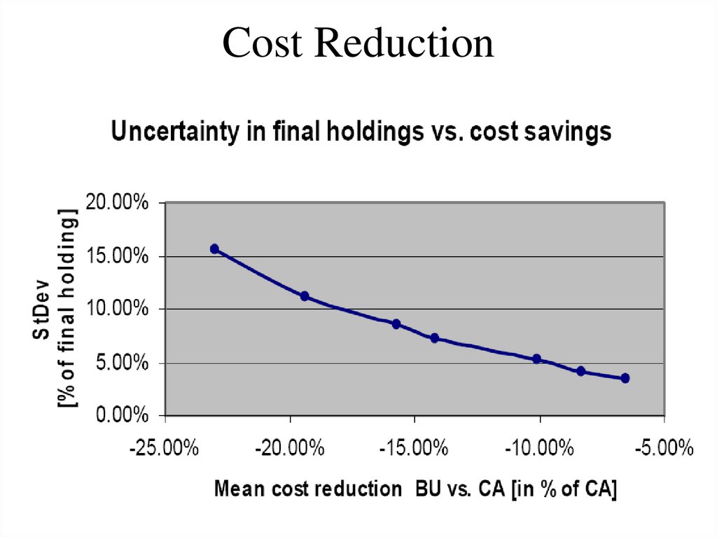
80. Cost Reduction

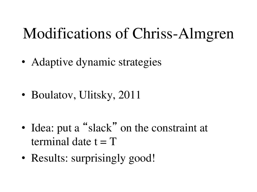
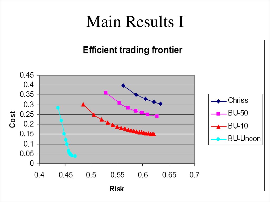
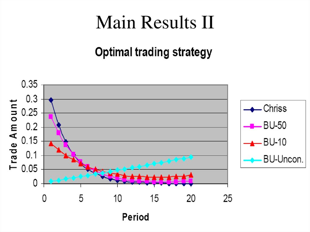
81. Modifications of Chriss-Almgren

• Adaptive dynamic strategies
• Boulatov, Ulitsky, 2011
• Idea: put a “slack” on the constraint at
terminal date t = T
• Results: surprisingly good!

82. Main Results I

83. Main Results II

84. Securities Trading when Liquidity Providers are Informed

Boulatov, George, 2011
84

85. Motivation

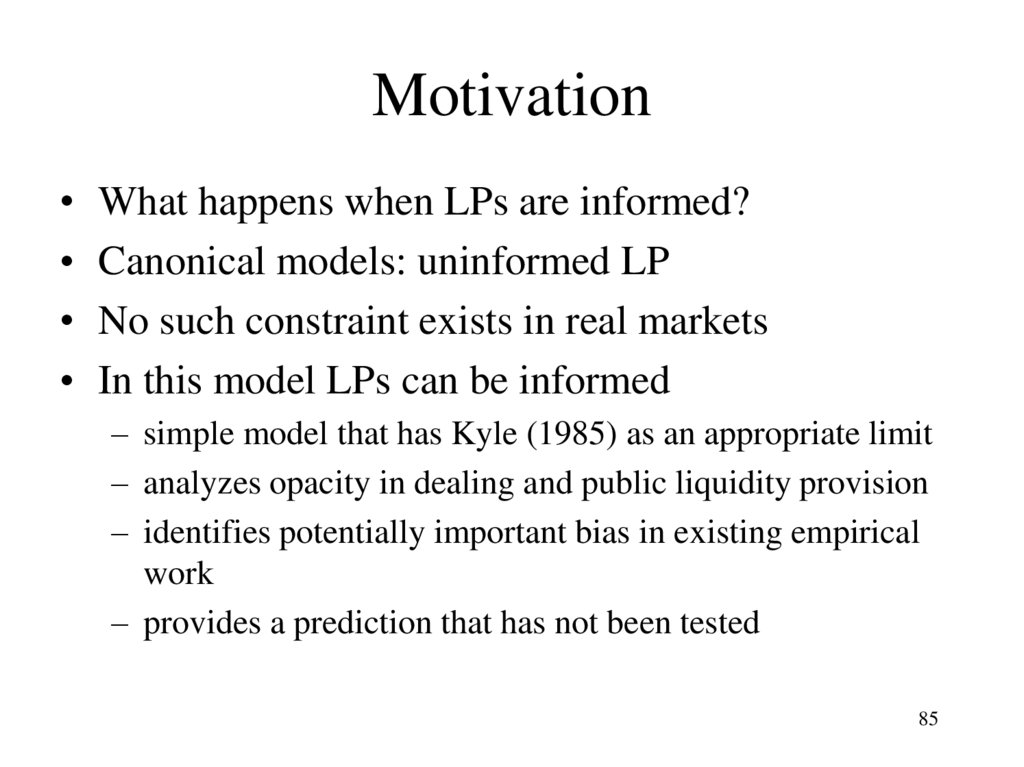
• What happens when LPs are informed?
• Canonical models: uninformed LP
• No such constraint exists in real markets
• In this model LPs can be informed
– simple model that has Kyle (1985) as an appropriate limit
– analyzes opacity in dealing and public liquidity provision
– identifies potentially important bias in existing empirical
work
– provides a prediction that has not been tested
85

86. This Model

• Based on Kyle ~ continuous price grid, traders compete
directly, order quantity unrestricted
• We consider two settings
– designated informed dealers
– informed traders choose to supply or demand liquidity
• Competition is more intense when the informed compete
as liquidity providers than liquidity demanders
86

87. Assumptions

• Single asset that pays off v~N(0, v2)
• J risk-neutral strategic liquidity providers who each
– observes a signal, sj, about the security’s payoff
– submits supply schedule yj(sj,p), where y>0 means sell, to a
consolidated “book” of orders
• N risk-neutral strategic liquidity demanders who each
– observes a signal, si, about the security’s payoff
– submits market order xi(si), where x>0 means buy, that is
executed against the consolidated “book” at a uniform price.
• What sj and si are, and whether N and J are exogenous or endogenous
varies across the settings we analyze.
• Uninformed liquidity traders submit market orders of u~N(0, u2)
87

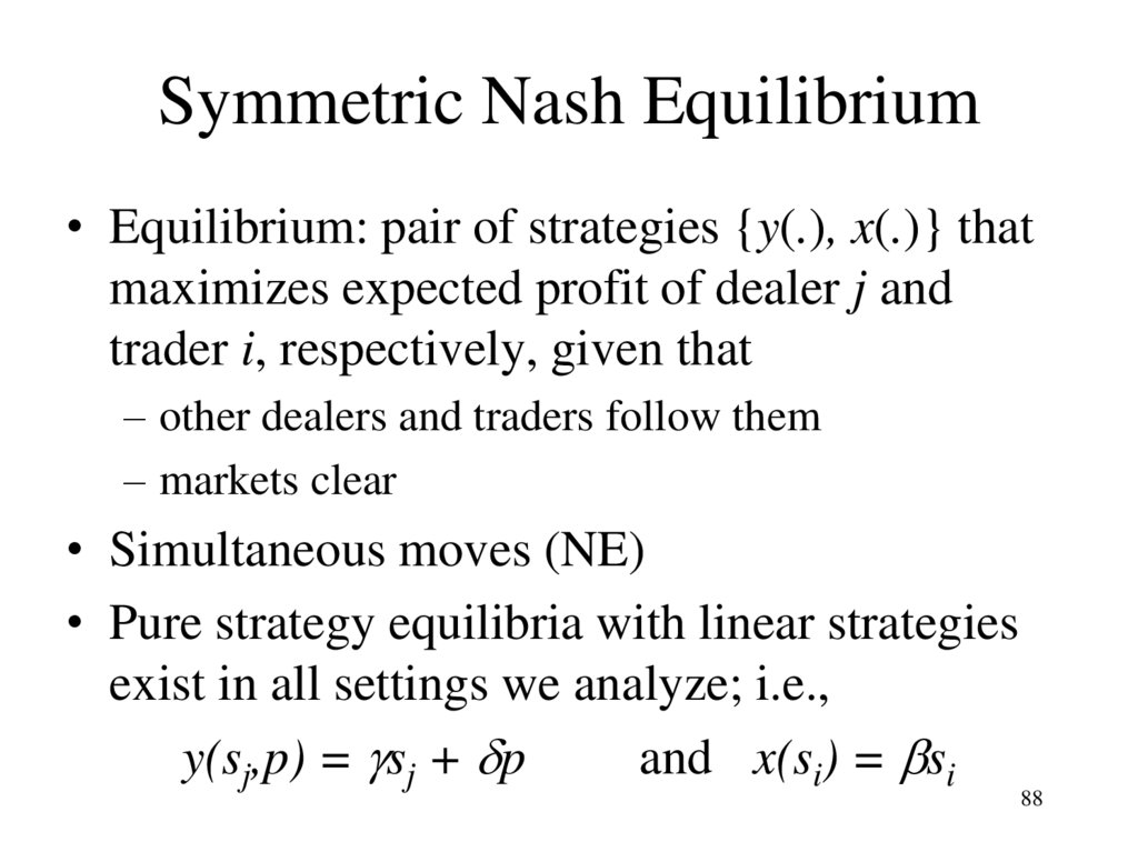
88. Symmetric Nash Equilibrium

• Equilibrium: pair of strategies {y(.), x(.)} that
maximizes expected profit of dealer j and
trader i, respectively, given that
– other dealers and traders follow them
– markets clear
• Simultaneous moves (NE)
• Pure strategy equilibria with linear strategies
exist in all settings we analyze; i.e.,
y(sj,p) = sj + p
and x(si) = si
88

89. Setting 1: Designated Dealers

• J dealers are designated by the market
• v = v1 + v2, components are indep. normal
• Dealers observe sj = v1 for all j
• If transparent, non-dealers are fully informed
and observe si = v
• If opaque, non-dealers are “blocked” from
observing v1 and observe only si = v2.
89

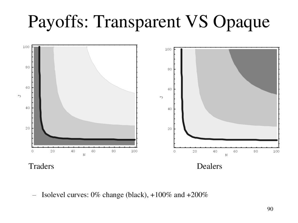
90. Payoffs: Transparent VS Opaque

100
100
80
80
60
J
J
60
40
40
20
20
0
20
Traders
40
N
60
80
100
0
20
40
N
60
80
100
Dealers
– Isolevel curves: 0% change (black), +100% and +200%
90

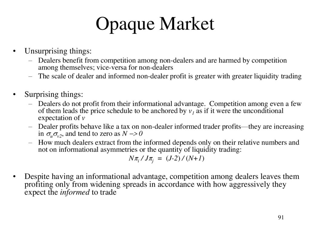
91. Opaque Market

Unsurprising things:
– Dealers benefit from competition among non-dealers and are harmed by competition
among themselves; vice-versa for non-dealers
– The scale of dealer and informed non-dealer profit is greater with greater liquidity trading
Surprising things:
– Dealers do not profit from their informational advantage. Competition among even a few
of them leads the price schedule to be anchored by v1 as if it were the unconditional
expectation of v
– Dealer profits behave like a tax on non-dealer informed trader profits—they are increasing
in u v2, and tend to zero as N > 0
– How much dealers extract from the informed depends only on their relative numbers and
not on informational asymmetries or the quantity of liquidity trading:
N i / J j = (J-2) / (N+1)
Despite having an informational advantage, competition among dealers leaves them
profiting only from widening spreads in accordance with how aggressively they
expect the informed to trade
91

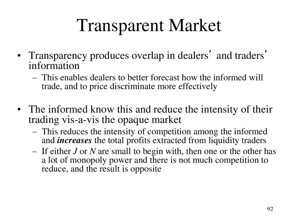
92. Transparent Market

• Transparency produces overlap in dealers’ and traders’
information
– This enables dealers to better forecast how the informed will
trade, and to price discriminate more effectively
• The informed know this and reduce the intensity of their
trading vis-a-vis the opaque market
– This reduces the intensity of competition among the informed
and increases the total profits extracted from liquidity traders
– If either J or N are small to begin with, then one or the other has
a lot of monopoly power and there is not much competition to
reduce, and the result is opposite
92

93. Results

• All informed choose to supply liquidity (J*=M) and
• Liquidity traders’ expected losses are minimized
– Competition is more intense when informed trade as LPs
than LDs
• Similar to Glosten’s (1994) conclusion on public
provision of liquidity except here
– Competition is imperfect
– Traders choose their order types
– In equilibrium the informed supply liqudity

94. Implications

• With the informed providing liquidity, the price
schedule reflects the security’s true value even
before crossing market orders
• Empirical Implication: More private
information “arrives” with limit rather than
market orders
– Consistent with evidence in Kaniel & Liu (2006)
and Rourke (2007)
– Existing measures of info content of trades are
biased downward

95. Empirical Evidence

• Hendershott, Jones & Menkveld (2008) compare
measures of market quality before and after Autoquote on
the NYSE
– Autoquote improved timeliness of information about trading
disseminated off the floor
• Quote midpoints move less in response to order arrivals
after Autoquote; i.e., price schedule better anticipates
order flow after Autoquote
• Dealers profit more after Autoquote
95

96. Setting 2: Endogenous Choice of Order Type

• M informed agents, each observes si = vi
• v = v1 + ... + vM
where vi ~ iid Normal
• M = J + N, where J is the number who
choose to submit supply schedules, N
choose market orders
• J* is such that no trader benefits by
switching order types
96

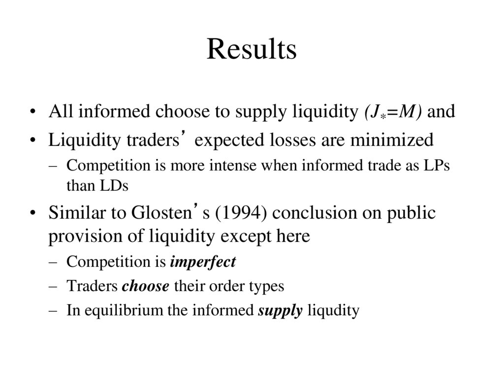
97. Results

• All informed choose to supply liquidity (J*=M) and
• Liquidity traders’ expected losses are minimized
– Competition is more intense when informed trade as LPs than
LDs
• Similar to Glosten’s (1994) conclusion on public provision
of liquidity except here
– Competition is imperfect
– Traders choose their order types
– In equilibrium the informed supply liqudity
97

98. Implications

• With the informed providing liquidity, the price
schedule reflects the security’s true value even
before crossing market orders
• Empirical Implication: More private
information “arrives” with limit rather than
market orders
– Consistent with evidence in Kaniel & Liu (2006)
and Rourke (2007)
– Existing measures of info content of trades are
98
biased downward

99. Adding friction to Liq. Provision

• Frictions drive informed away from liquidity
provision and toward demanding liquidity
• Breaching anonymity: partial loss of LPs’ info.
advantage (similar to Foucault, et.al. ’07)
• Other frictions would have a similar effect
– Direct costs of monitoring limit orders (Seppi, ’97)
– Delay in cancellation of previous orders features
prominently in dynamic model of Goettler, et.al. ’07

100. Results

• Greater anonymity breach -- more migration from
liquidity provision to liquidity demand
– Greater friction causes more migration
• The more informed there are, the smaller is the
anonymity breach necessary to cause migration
– Frictions have bigger impacts, the greater the intensity of
potential competition
• Anonymity promotes competition
• New Empirical Prediction: More info “arrives” with
limit than market orders in markets that are more
protective of LPs anonymity

101. Equilibrium number of liquidity providers

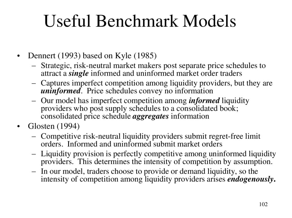
102. Useful Benchmark Models

• Dennert (1993) based on Kyle (1985)
– Strategic, risk-neutral market makers post separate price schedules to
attract a single informed and uninformed market order traders
– Captures imperfect competition among liquidity providers, but they are
uninformed. Price schedules convey no information
– Our model has imperfect competition among informed liquidity
providers who post supply schedules to a consolidated book;
consolidated price schedule aggregates information
• Glosten (1994)
– Competitive risk-neutral liquidity providers submit regret-free limit
orders. Informed and uninformed submit market orders
– Liquidity provision is perfectly competitive among uninformed liquidity
providers. This determines the intensity of competition by assumption.
– In our model, traders choose to provide or demand liquidity, so the
intensity of competition among liquidity providers arises endogenously.
102

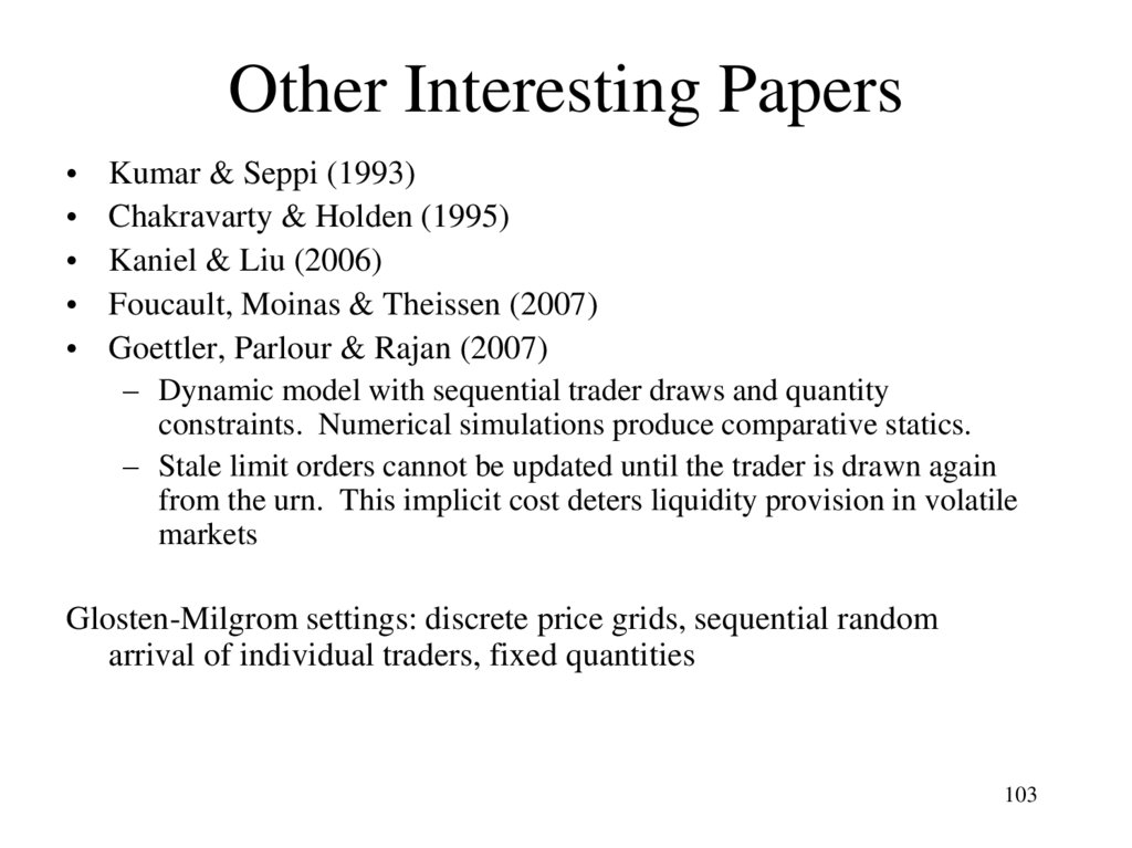
103. Other Interesting Papers

Kumar & Seppi (1993)
Chakravarty & Holden (1995)
Kaniel & Liu (2006)
Foucault, Moinas & Theissen (2007)
Goettler, Parlour & Rajan (2007)
– Dynamic model with sequential trader draws and quantity
constraints. Numerical simulations produce comparative statics.
– Stale limit orders cannot be updated until the trader is drawn again
from the urn. This implicit cost deters liquidity provision in volatile
markets
Glosten-Milgrom settings: discrete price grids, sequential random
arrival of individual traders, fixed quantities
103

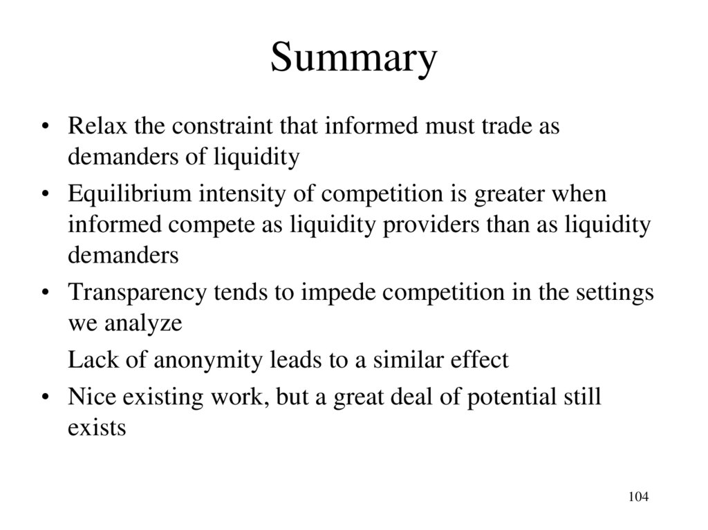
104. Summary

• Relax the constraint that informed must trade as
demanders of liquidity
• Equilibrium intensity of competition is greater when
informed compete as liquidity providers than as liquidity
demanders
• Transparency tends to impede competition in the settings
we analyze
Lack of anonymity leads to a similar effect
• Nice existing work, but a great deal of potential still
exists
104

105. Limited Dealer Attention and Quote Adjustments

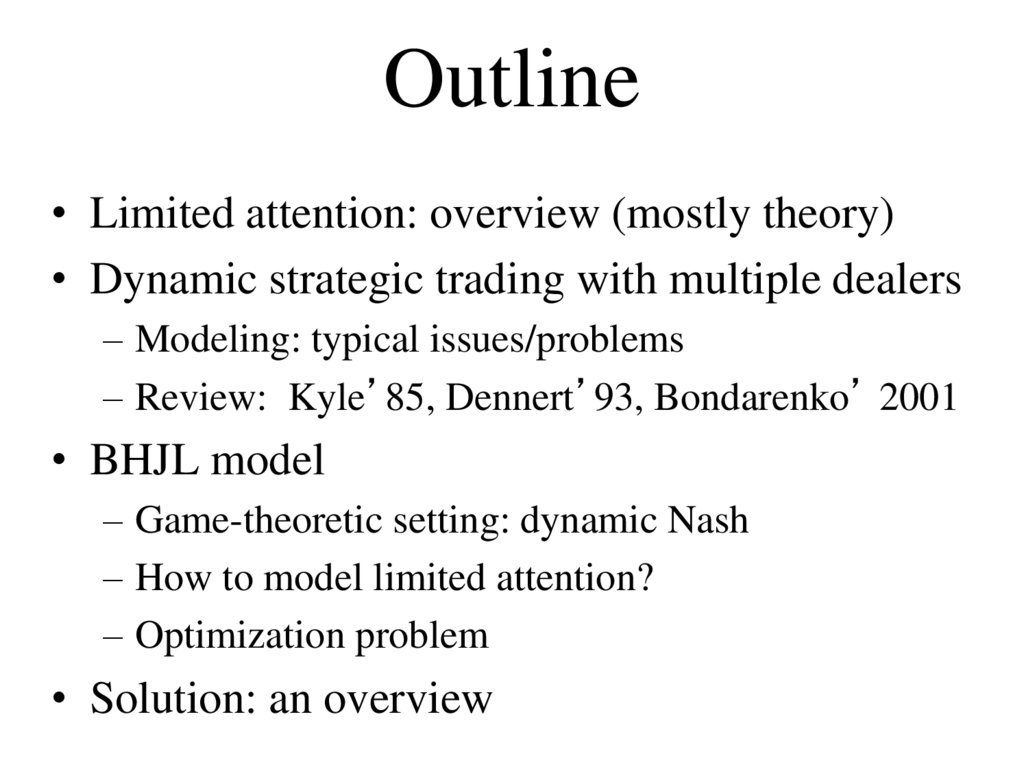
Boulatov, Hatch, Johnson, Lei (BHJL), 2007

106. Outline

• Limited attention: overview (mostly theory)
• Dynamic strategic trading with multiple dealers
– Modeling: typical issues/problems
– Review: Kyle’85, Dennert’93, Bondarenko’ 2001
• BHJL model
– Game-theoretic setting: dynamic Nash
– How to model limited attention?
– Optimization problem
• Solution: an overview

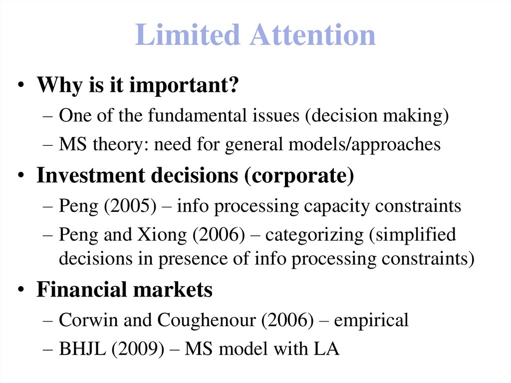
107. Limited Attention

• Why is it important?
– One of the fundamental issues (decision making)
– MS theory: need for general models/approaches
• Investment decisions (corporate)
– Peng (2005) – info processing capacity constraints
– Peng and Xiong (2006) – categorizing (simplified
decisions in presence of info processing constraints)
• Financial markets
– Corwin and Coughenour (2006) – empirical
– BHJL (2009) – MS model with LA

108. References I

• Alex Boulatov, Brian C. Hatch, Shane A. Johnson, Adam Y.C.
Lei, 2009, “Dealer Attention, the Speed of Quote Adjustment
to Information, and Net Dealer Revenue”, Journal of Banking
and Finance, forthcoming.
• Lin Peng, 2005, “Learning with Information Capacity
Constraints”, Journal of Financial and Quantitative Analysis,
40, 307-329.
• Shane Corwin and Jay Coughenour, 2008, “Limited Attention
and the Allocation of Effort in Securities Trading", Journal of
Finance, forthcoming.
• Lin Peng and Wei Xiong, 2006, “Investor Attention,
Overconfidence and Category Learning”, Journal of Financial
Economics, 80, 563-602.

109. References II

• Albert S. Kyle, 1985, “Continuous Auctions and Informed
Trader Trading”, Econometrica 53, 1315-1335.
• Oleg Bondarenko, 2001, “Competing market makers, liquidity
provisions, and bid-ask spreads”, Journal of Financial Markets
4, 269-308.
• Jürgen Dennert, 1993, “Price Competition between Market
Makers”, Review of Economic Studies 60, 735-751.

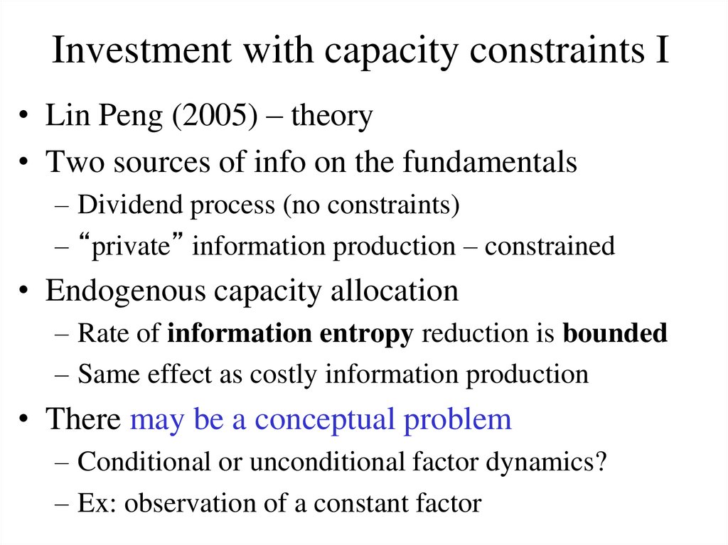
110. Investment with capacity constraints I

• Lin Peng (2005) – theory
• Two sources of info on the fundamentals
– Dividend process (no constraints)
– “private” information production – constrained
• Endogenous capacity allocation
– Rate of information entropy reduction is bounded
– Same effect as costly information production
• There may be a conceptual problem
– Conditional or unconditional factor dynamics?
– Ex: observation of a constant factor

111. Investment with capacity constraints II

• Endogenous capacity allocation: results
• Allocate more capacity to
– Large stocks
– Stocks with higher uncertainty
• Note: both are perfectly consistent with BHJL
• Results (cross-section)
– Higher rate of adjustment to fundamental shocks
– Lower residual uncertainty

112. Implications for financial markets I

• Corwin and Coughenour (2008) – Empirical
• Evidence on NYSE specialists (market-makers)
– Why limited attention? Time & processing constraints
• Allocate more attention to
– More “active” stocks (higher trading activity)
• Results
– Lower transaction costs
– Higher liquidity
• Note: all the above is consistent with BHJL

113. Implications for financial markets II

• Why NYSE? Specialists: well-defined portfolios
• Limited Attention Hypothesis
“If limited attention forces a specialist to allocate
efforts across stocks, we expect their ability to
provide liquidity for a given stock to be
negatively related to the attention requirements of
other stocks in their portfolio…”
• Testing LAH
– intraday TAQ + trading floor location data
– Results: BA spreads decrease, rate and magnitude of
price improvements increase in attention

114. Strategic trading and liquidity provision

• Strategic nature of insider trading
• Lifting the market efficiency condition:
– Dealers are making profits (imperfect
competition)
• two-sided strategic trading (Dennert’93)

115. BHJL: Limited Dealers’ Attention

• Limited attention – slow reaction to new info
• Focus on dynamics of quote adjustment process
• “A dealer who is slow to detect and incorporate new
information into quoted prices faces the risk that on
subsequent trades he buys from (sells to) informed
traders or even liquidity traders at prices that are too
high (low).”
• Therefore, dealer with higher attention rate should
(ceteris paribus) make higher expected profits.
• Note: competition with other dealers and insiders

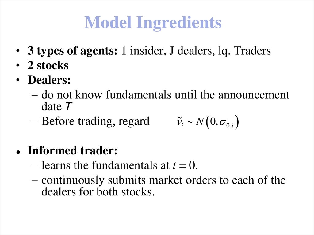
116. Model Ingredients

• 3 types of agents: 1 insider, J dealers, lq. Traders
• 2 stocks
• Dealers:
– do not know fundamentals until the announcement
date T
vi ~ N 0, 0,i
– Before trading, regard
Informed trader:
– learns the fundamentals at t = 0.
– continuously submits market orders to each of the
dealers for both stocks.

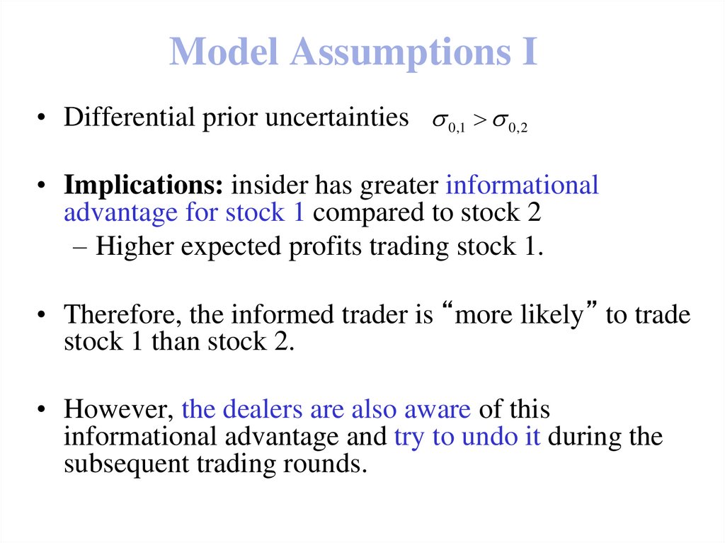
117. Model Assumptions I

• Differential prior uncertainties 0,1 > 0,2
• Implications: insider has greater informational
advantage for stock 1 compared to stock 2
– Higher expected profits trading stock 1.
• Therefore, the informed trader is “more likely” to trade
stock 1 than stock 2.
• However, the dealers are also aware of this
informational advantage and try to undo it during the
subsequent trading rounds.

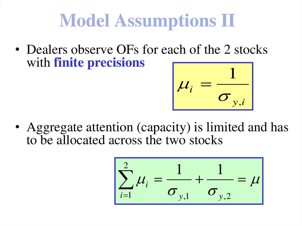
118. Model Assumptions II

• Dealers observe OFs for each of the 2 stocks
with finite precisions
i
1
y ,i
• Aggregate attention (capacity) is limited and has
to be allocated across the two stocks
2
1
i 1
i
y ,1
1
y,2

119. Attendance parameters

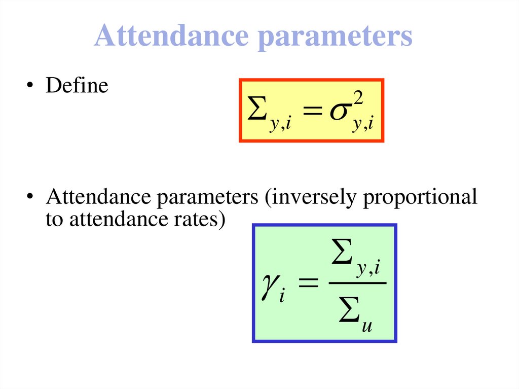
• Define
y ,i
2
y ,i
• Attendance parameters (inversely proportional
to attendance rates)
i
y ,i
u

120. Optimal Attention Allocation

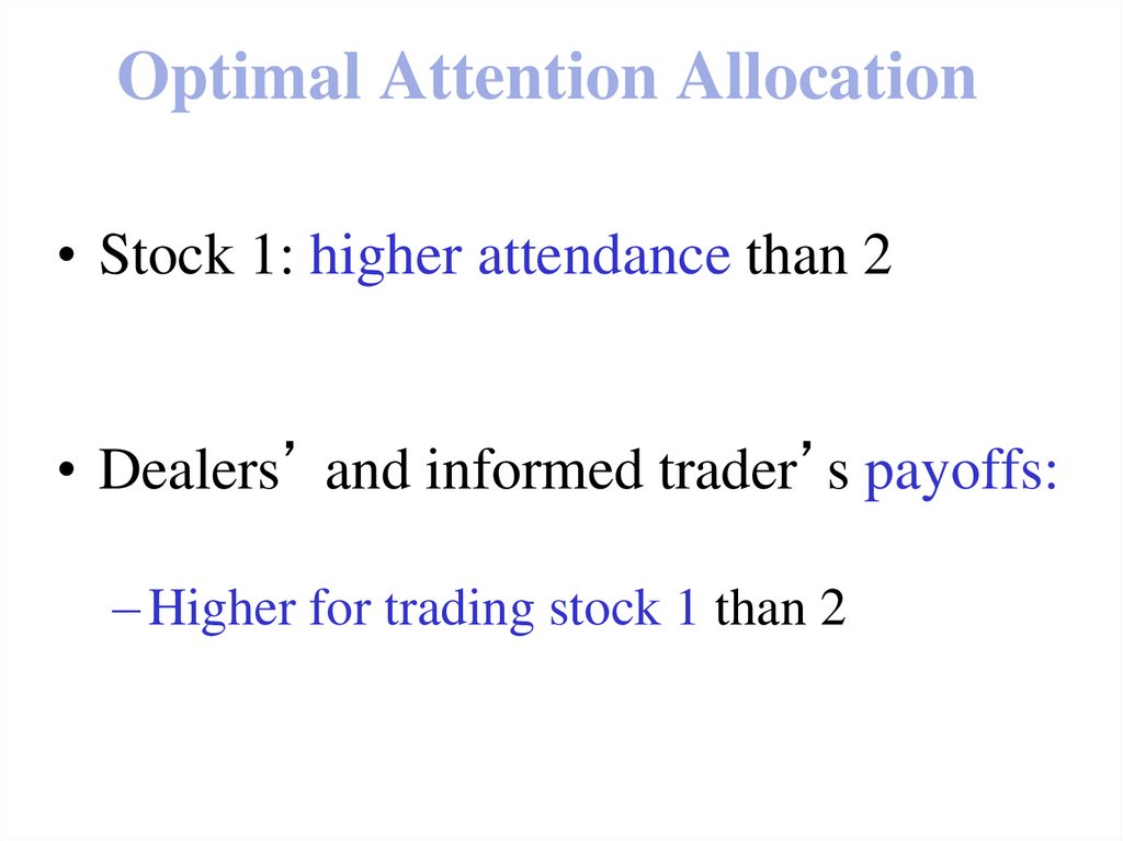
• Stock 1: higher attendance than 2
• Dealers’ and informed trader’s payoffs:
– Higher for trading stock 1 than 2

121. Multiple oligopolistic dealers

• Insider’s problem: reaction function
T
2
I max E dt k t v Pk t
max
X k ( )
k ( )
0
J
1
1
Xk
X;
k
k 1 k
• Dealers: price is greater than ME
dPk k t dyk ; d D ,k E dyk Pk vk
• Equilibrium:
J 2 *
*
t J J
0 ; 0 const
J 1
*
k
*

122. Model: Details

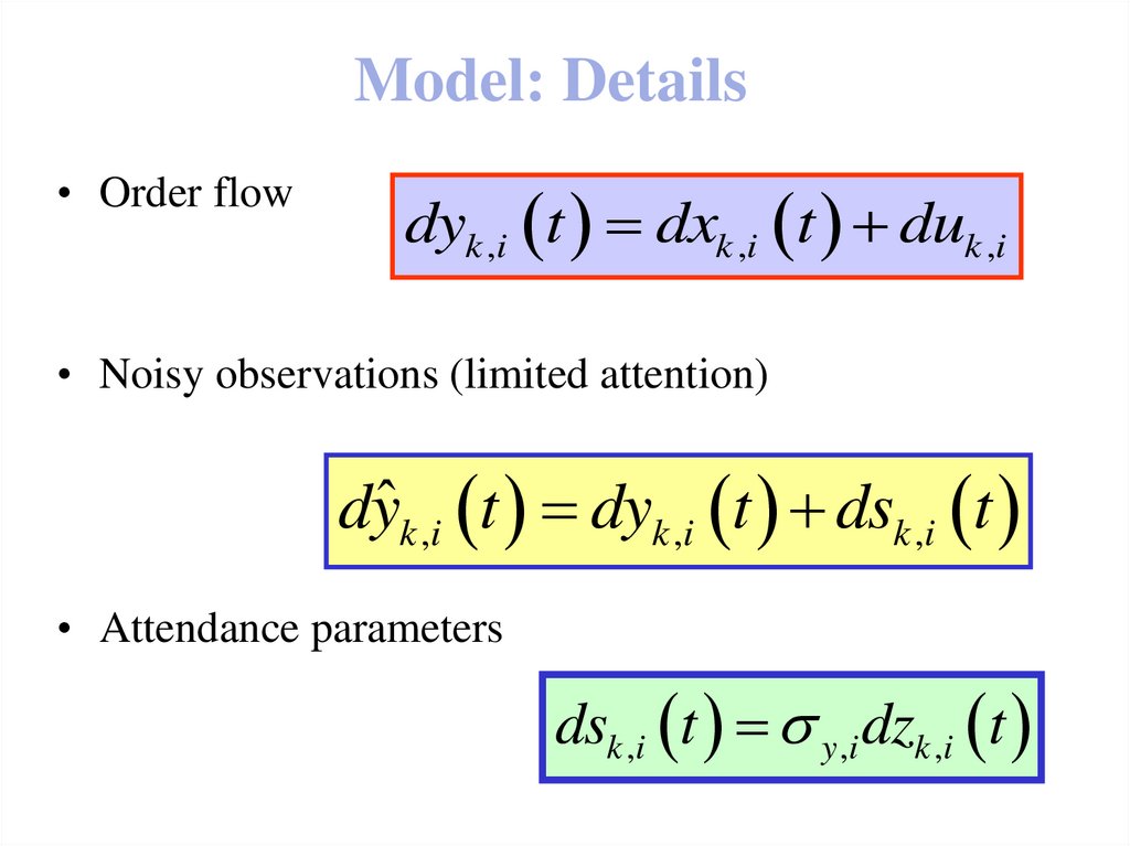
• Order flow
dyk ,i t dxk ,i t duk ,i
• Noisy observations (limited attention)
dyˆk ,i t dyk ,i t dsk ,i t
• Attendance parameters
dsk ,i t y ,i dzk ,i t

123. Model: Strategies

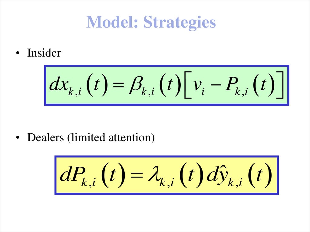
• Insider
dxk ,i t k ,i t vi Pk ,i t
• Dealers (limited attention)
dPk ,i t k ,i t dyˆk ,i t

124. Optimization

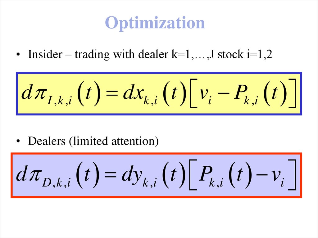
• Insider – trading with dealer k=1,…,J stock i=1,2
d I , k ,i t dxk ,i t vi Pk ,i t
• Dealers (limited attention)
d D , k ,i t dyk ,i t Pk ,i t vi

125. Equilibrium I

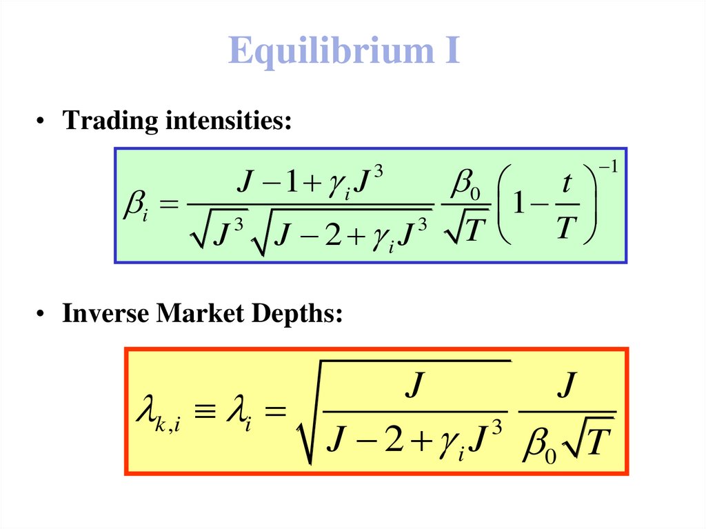
• Trading intensities:
i
J 1 i J
J
3
0
3
J 2 iJ
3
t
1
T T
1
• Inverse Market Depths:
k ,i i
J
J
3
J 2 i J 0 T

126. Equilibrium II

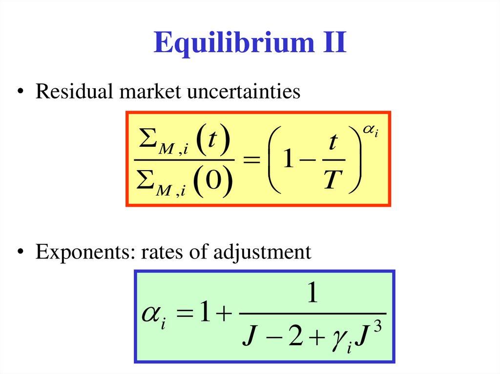
• Residual market uncertainties
M ,i t
i
t
1
M ,i 0
T
• Exponents: rates of adjustment
1
i 1
3
J 2 iJ

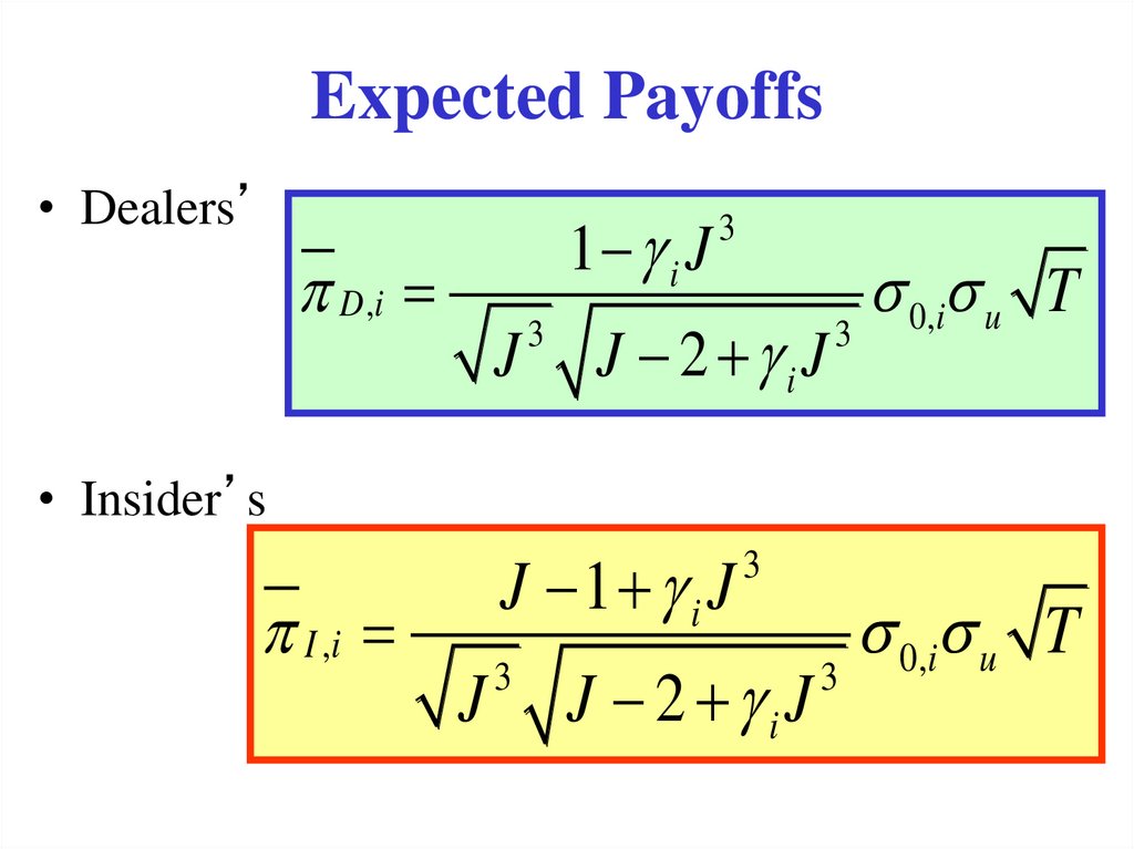
127. Expected Payoffs

• Dealers’
1 i J
D ,i
J
3
3
J 2 iJ
3
0,i u T
• Insider’s
J 1 i J
I ,i
J
3
3
J 2 iJ
3
0,i u T

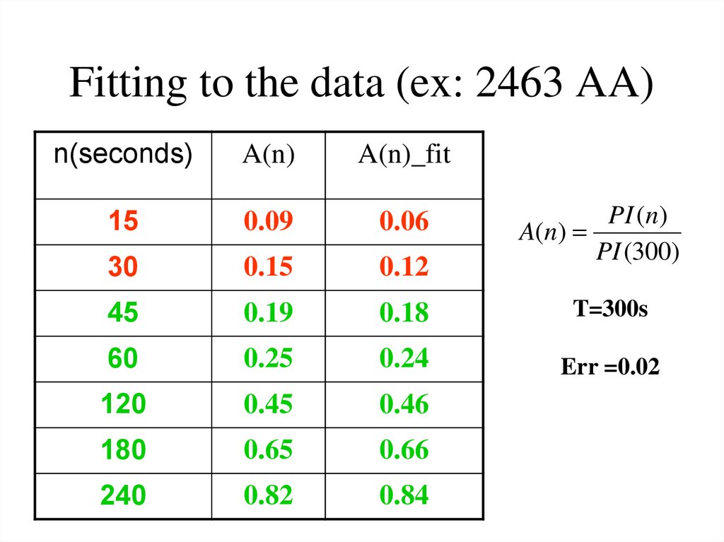
128. Fitting to the data (ex: 2463 AA)

n(seconds)
A(n)
A(n)_fit
15
0.09
0.06
30
0.15
0.12
45
0.19
0.18
T=300s
60
0.25
0.24
Err =0.02
120
0.45
0.46
180
0.65
0.66
240
0.82
0.84
PI (n)
A(n)
PI (300)

129. Conclusions

• Dynamic Bayesian Nash CT linear equilibrium
– Same in Nash and Stackelberg cases
• Fitting to the data: fits reasonably well