Convolutional neural networks (CNNs)

1.

Convolutional neural
networks (CNNs)
Faculty of Engineering and
Natural Sciences

2.

Contents
● Introduction
● Basic building blocks
● Architecture
● Parameter sharing &
sparsity
● Popular architectures
● Training CNNs
● Regularization techniques
● Conclusion

3.

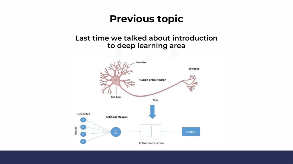
Previous topic
Last time we talked about introduction
to deep learning area

4.

Introduction to CNNs

5.

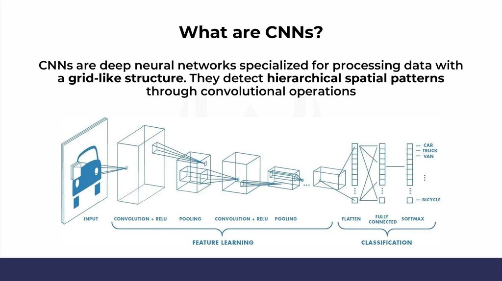
What are CNNs?
CNNs are deep neural networks specialized for processing data with
a grid-like structure. They detect hierarchical spatial patterns
through convolutional operations

6.

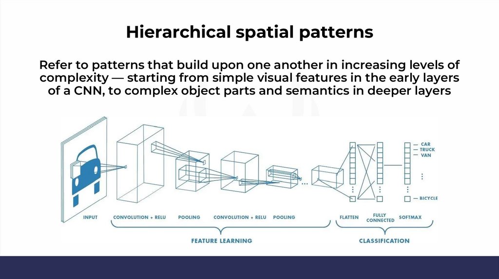
Hierarchical spatial patterns
Refer to patterns that build upon one another in increasing levels of
complexity — starting from simple visual features in the early layers
of a CNN, to complex object parts and semantics in deeper layers

7.

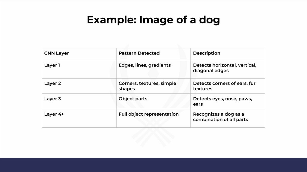
Example: Image of a dog
CNN Layer
Pattern Detected
Description
Layer 1
Edges, lines, gradients
Detects horizontal, vertical,
diagonal edges
Layer 2
Corners, textures, simple
shapes
Detects corners of ears, fur
textures
Layer 3
Object parts
Detects eyes, nose, paws,
ears
Layer 4+
Full object representation
Recognizes a dog as a
combination of all parts

8.

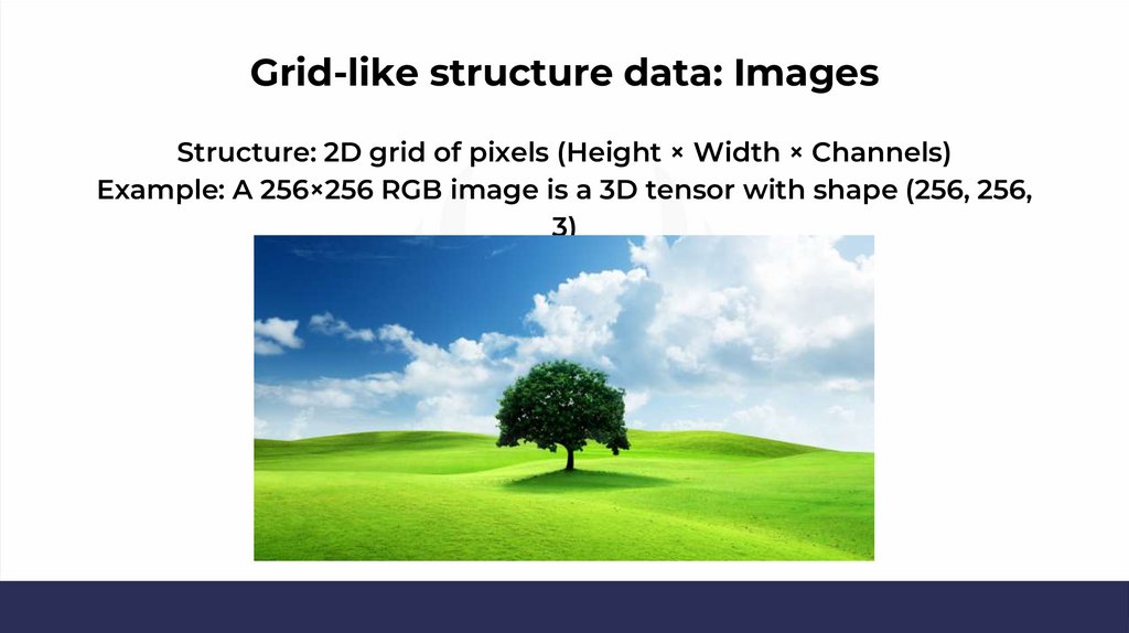
Grid-like structure data: Images
Structure: 2D grid of pixels (Height × Width × Channels)
Example: A 256×256 RGB image is a 3D tensor with shape (256, 256,
3)

9.

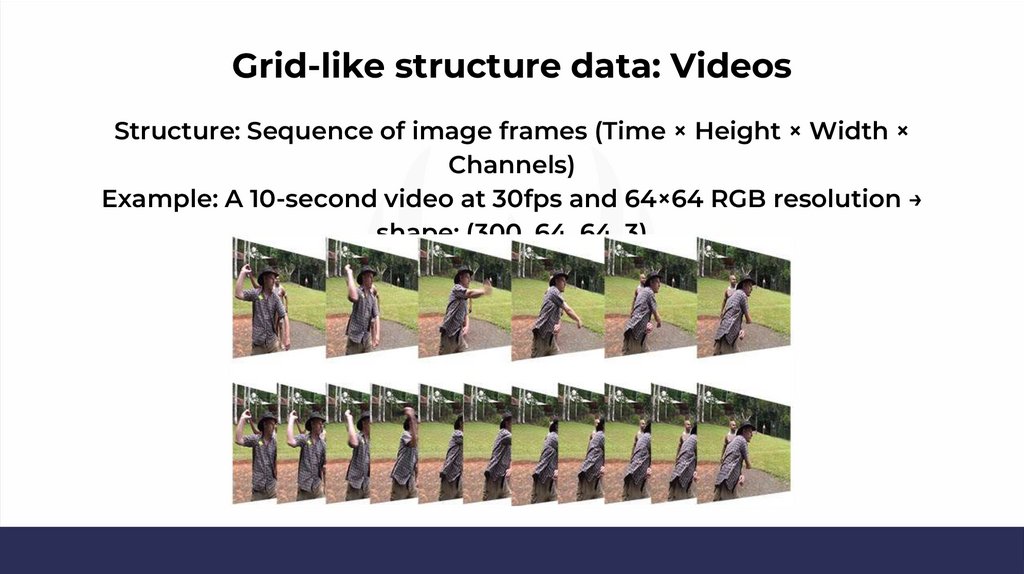
Grid-like structure data: Videos
Structure: Sequence of image frames (Time × Height × Width ×
Channels)
Example: A 10-second video at 30fps and 64×64 RGB resolution →
shape: (300, 64, 64, 3)

10.

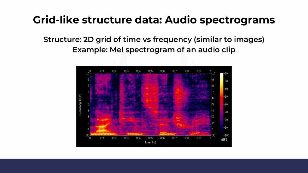
Grid-like structure data: Audio spectrograms
Structure: 2D grid of time vs frequency (similar to images)
Example: Mel spectrogram of an audio clip

11.

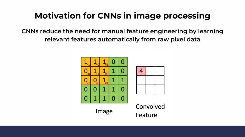
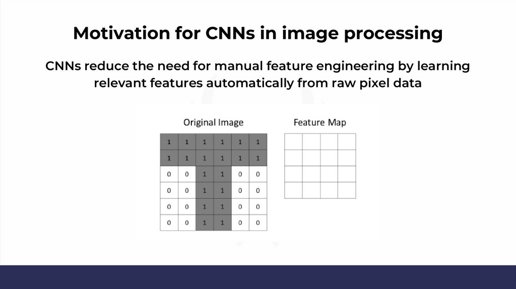
Motivation for CNNs in image processing
CNNs reduce the need for manual feature engineering by learning
relevant features automatically from raw pixel data

12.

Motivation for CNNs in image processing
CNNs reduce the need for manual feature engineering by learning
relevant features automatically from raw pixel data

13.

Basic building blocks

14.

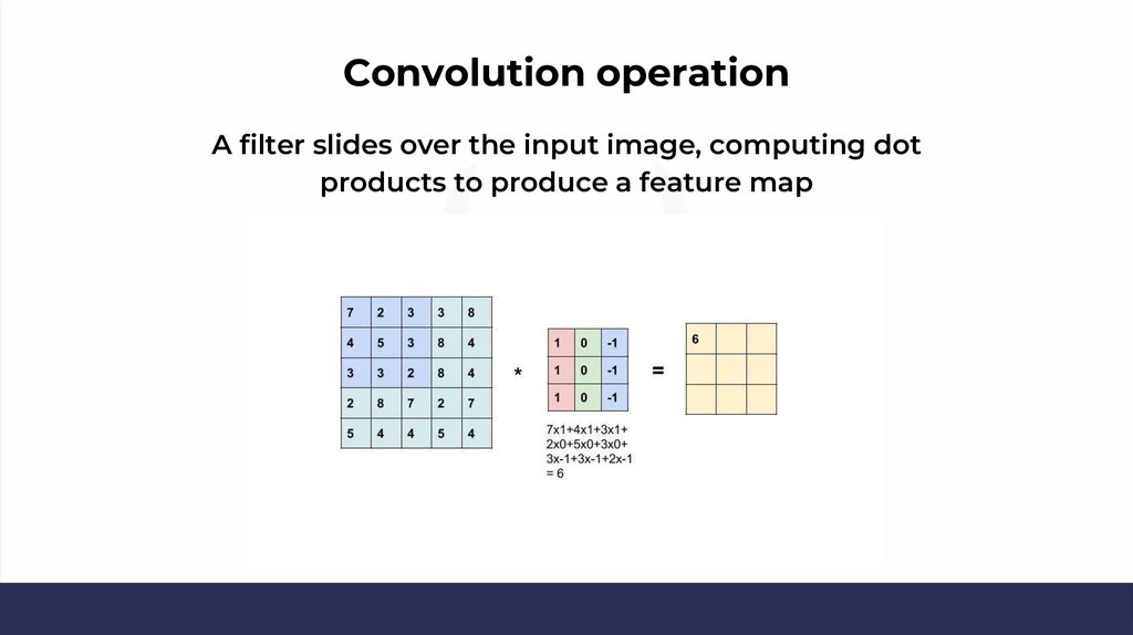
Convolution operation
A filter slides over the input image, computing dot
products to produce a feature map

15.

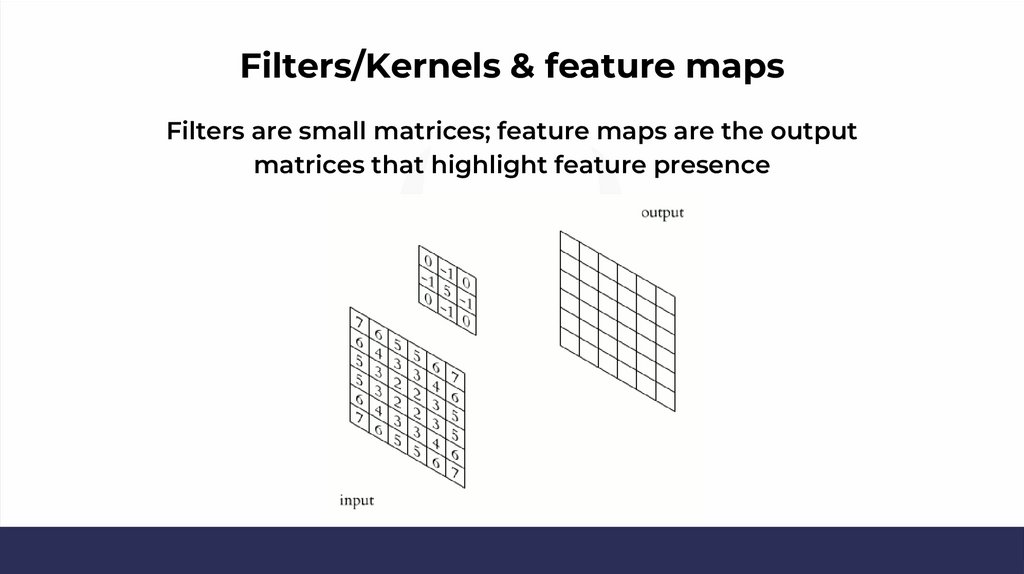
Filters/Kernels & feature maps
Filters are small matrices; feature maps are the output
matrices that highlight feature presence

16.

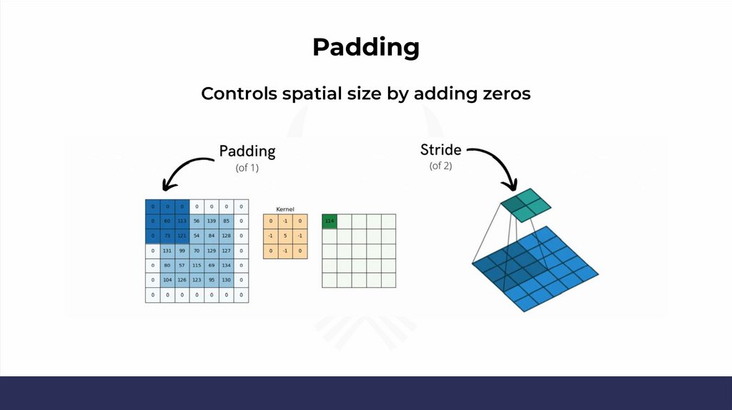
Padding
Controls spatial size by adding zeros

17.

Stride
Determines step size of filter movement

18.

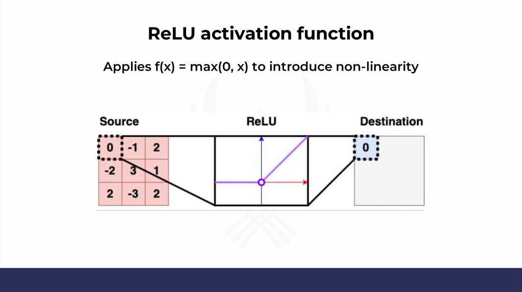
ReLU activation function
Applies f(x) = max(0, x) to introduce non-linearity

19.

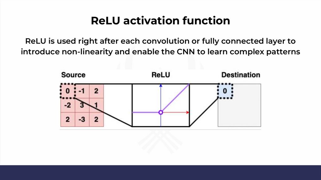
ReLU activation function
ReLU is used right after each convolution or fully connected layer to
introduce non-linearity and enable the CNN to learn complex patterns

20.

CNN architecture

21.

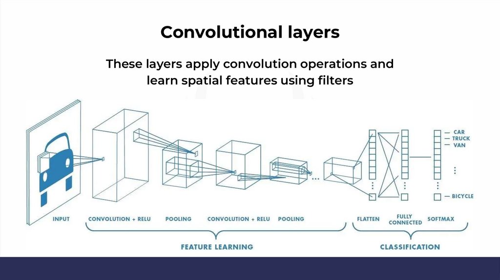
Convolutional layers
These layers apply convolution operations and
learn spatial features using filters

22.

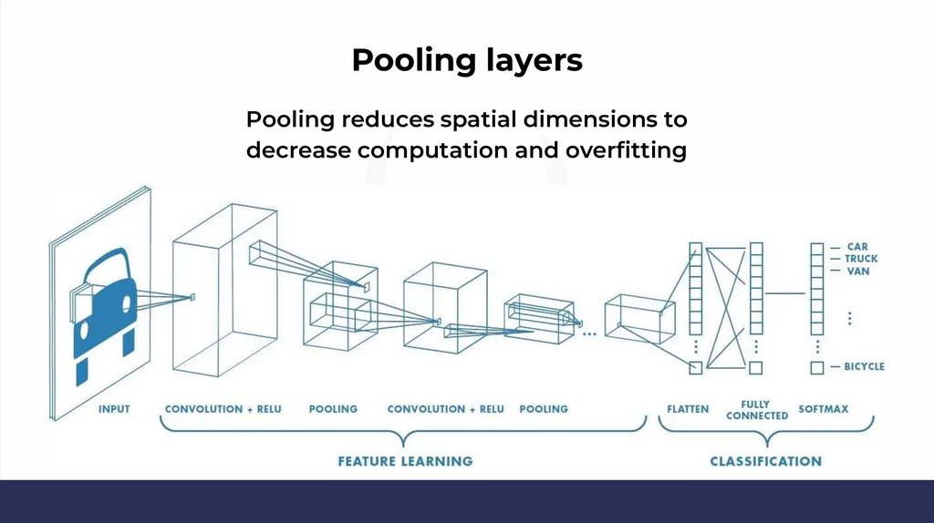
Pooling layers
Pooling reduces spatial dimensions to
decrease computation and overfitting

23.

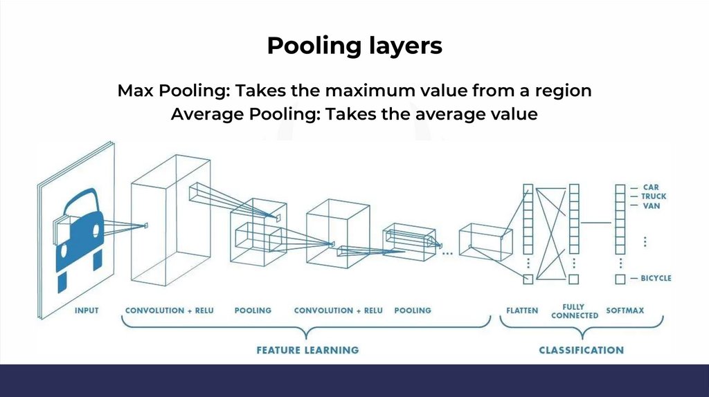
Pooling layers
Max Pooling: Takes the maximum value from a region
Average Pooling: Takes the average value

24.

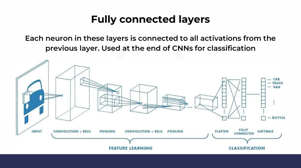
Fully connected layers
Each neuron in these layers is connected to all activations from the
previous layer. Used at the end of CNNs for classification

25.

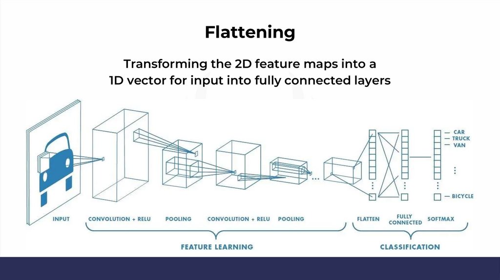
Flattening
Transforming the 2D feature maps into a
1D vector for input into fully connected layers

26.

Parameter sharing & sparsity

27.

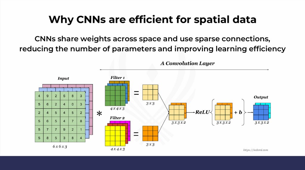
Why CNNs are efficient for spatial data
CNNs share weights across space and use sparse connections,
reducing the number of parameters and improving learning efficiency

28.

Popular CNN architectures

29.

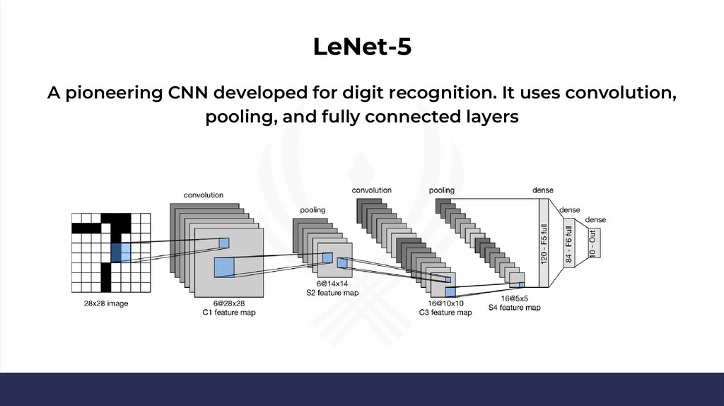
LeNet-5
A pioneering CNN developed for digit recognition. It uses convolution,
pooling, and fully connected layers

30.

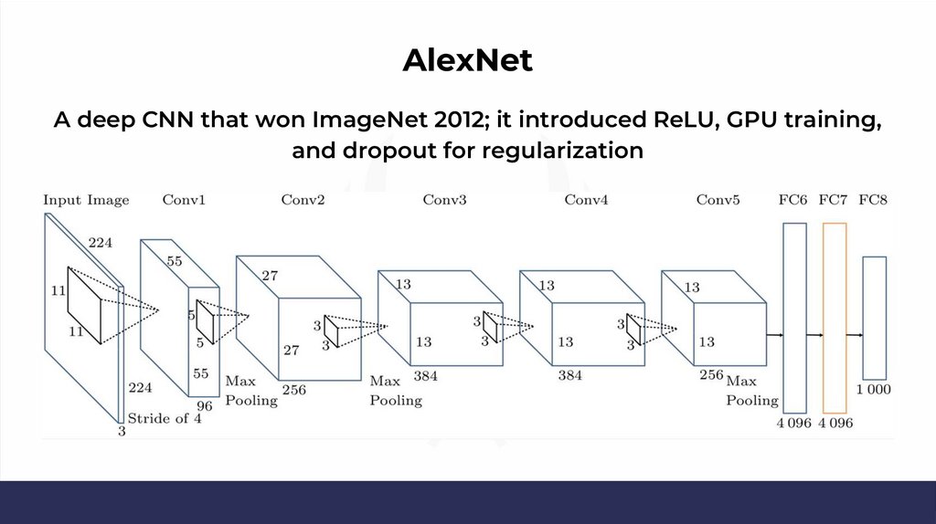
AlexNet
A deep CNN that won ImageNet 2012; it introduced ReLU, GPU training,
and dropout for regularization

31.

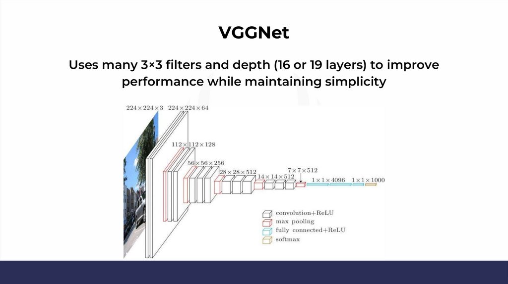
VGGNet
Uses many 3×3 filters and depth (16 or 19 layers) to improve
performance while maintaining simplicity

32.

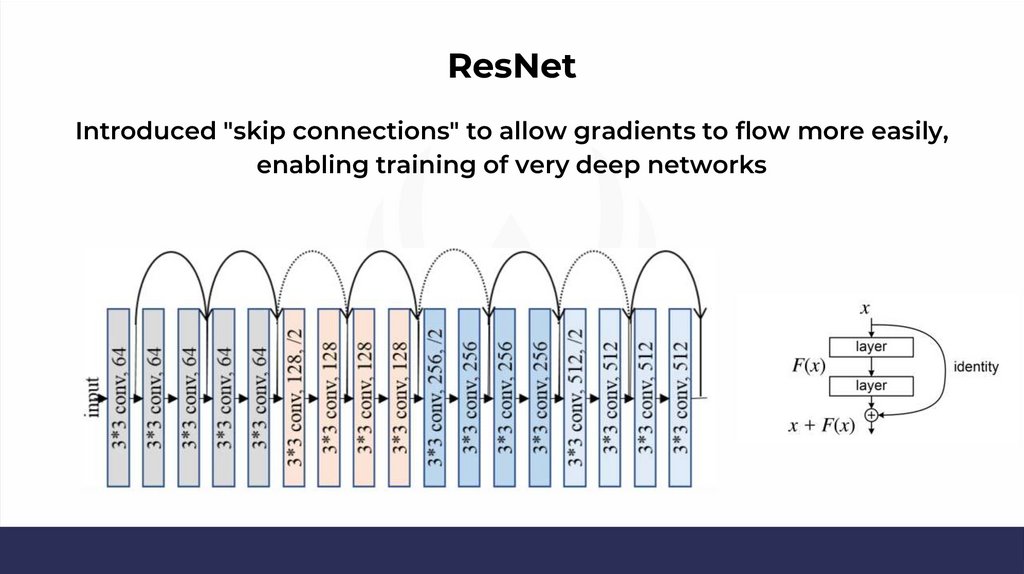
ResNet
Introduced "skip connections" to allow gradients to flow more easily,
enabling training of very deep networks

33.

Training CNNs

34.

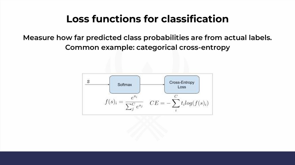
Loss functions for classification
Measure how far predicted class probabilities are from actual labels.
Common example: categorical cross-entropy

35.

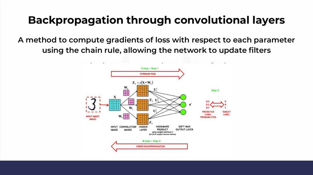
Backpropagation through convolutional layers
A method to compute gradients of loss with respect to each parameter
using the chain rule, allowing the network to update filters

36.

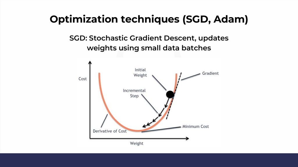
Optimization techniques (SGD, Adam)
SGD: Stochastic Gradient Descent, updates
weights using small data batches

37.

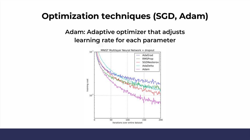
Optimization techniques (SGD, Adam)
Adam: Adaptive optimizer that adjusts
learning rate for each parameter

38.

Regularization techniques

39.

Dropout
Randomly deactivates neurons
during training to prevent overfitting

40.

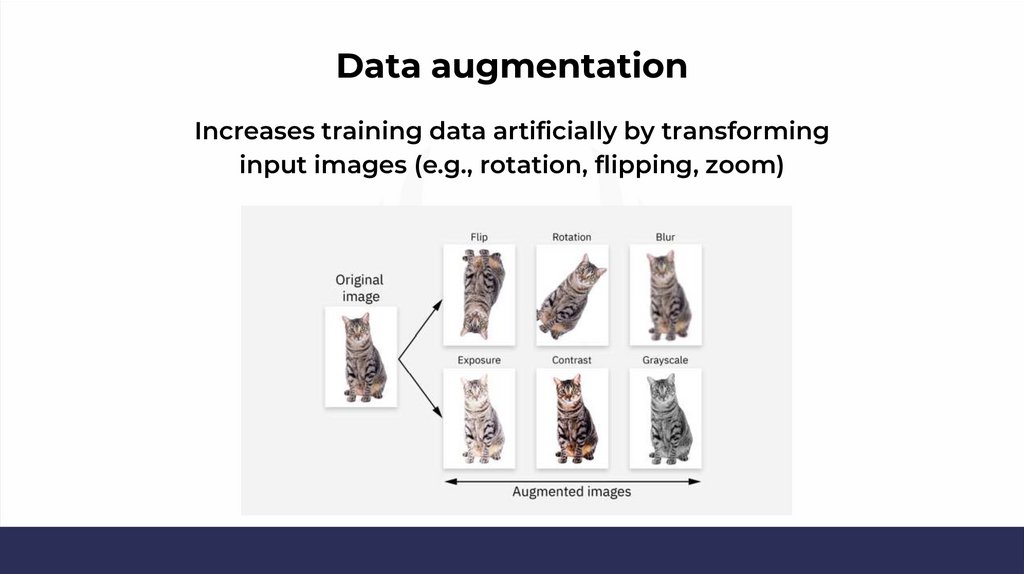
Data augmentation
Increases training data artificially by transforming
input images (e.g., rotation, flipping, zoom)

41.

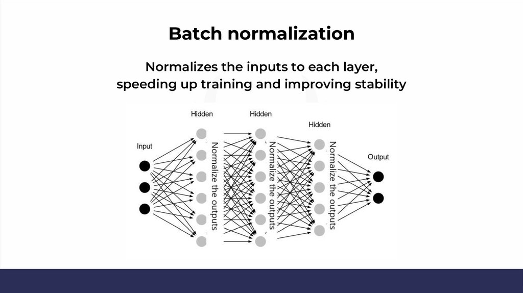
Batch normalization
Normalizes the inputs to each layer,
speeding up training and improving stability

42.

CNNs in practice

43.

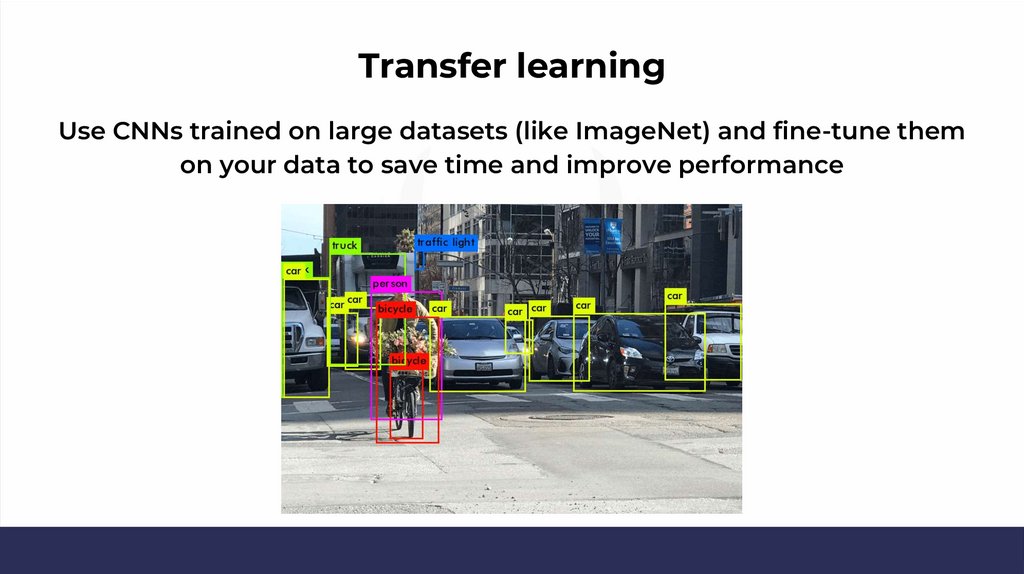
Transfer learning
Use CNNs trained on large datasets (like ImageNet) and fine-tune them
on your data to save time and improve performance

44.

Limitations & Challenges

45.

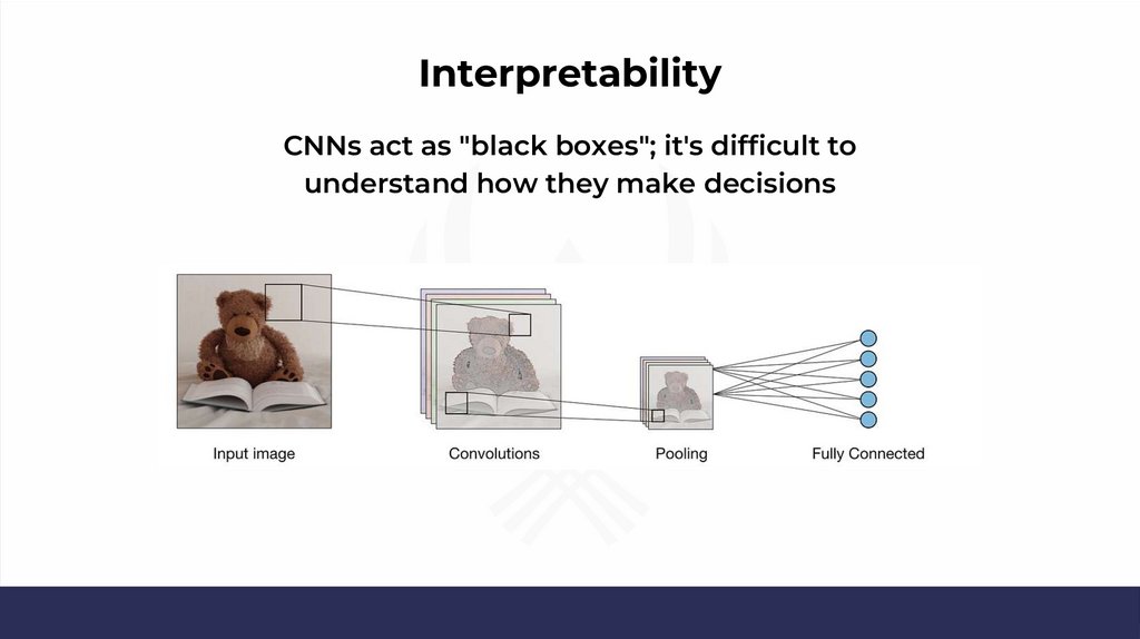
Interpretability
CNNs act as "black boxes"; it's difficult to
understand how they make decisions

46.

Computational cost
Training CNNs requires significant
GPU resources and time

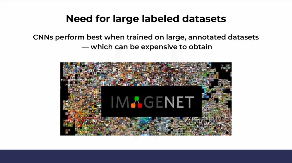
47.

Need for large labeled datasets
CNNs perform best when trained on large, annotated datasets
— which can be expensive to obtain

48.

Q/A Session