Production function

1. Production Function

Factors of production:
• Land
• Labour
• Capital
• Organization
Production Function
Q = f (Land, Labour, Capital, Organization)
Q = f (L, L, C, O)
Cobb Douglas Production Function
Q = f (K, L)
Q = A Kα Lβ
Q = the maximum rate of output for a given rate of capital (K) and labour (L)

2. Production Function

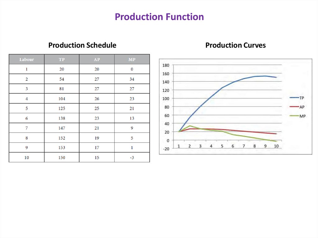
Total production (TP) - the maximum level of output that can be produced
with a given amount of input.
Average Production (AP) - output produced per unit of input AP = Q/L
Marginal Production (MP) - change in total output produced by the last
unit of an input
Marginal production of labour = Δ Q / Δ L (i.e. change in the quantity
produced to a given change in the labour)
Marginal production of capital = Δ Q / Δ K (i.e. change in the quantity
produced to a given change in the capital)

3. Production Function

Production Schedule
Production Curves

4. Production Function:

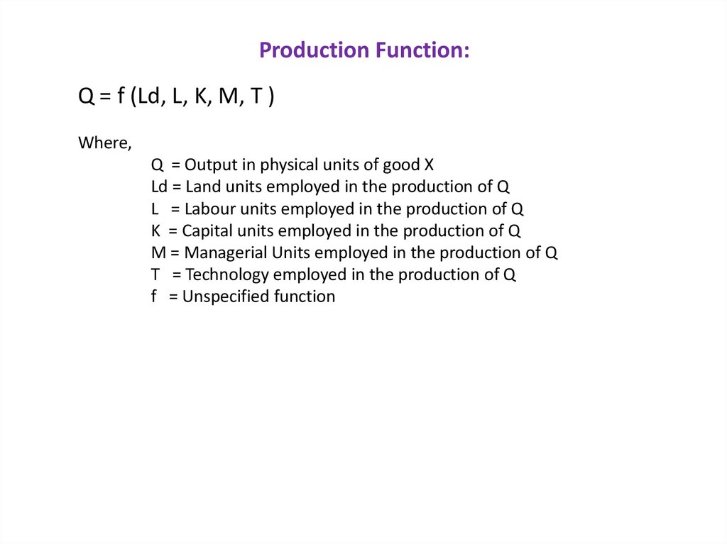
Q = f (Ld, L, K, M, T )
Where,
Q = Output in physical units of good X
Ld = Land units employed in the production of Q
L = Labour units employed in the production of Q
K = Capital units employed in the production of Q
M = Managerial Units employed in the production of Q
T = Technology employed in the production of Q
f = Unspecified function

5. The law of diminishing returns

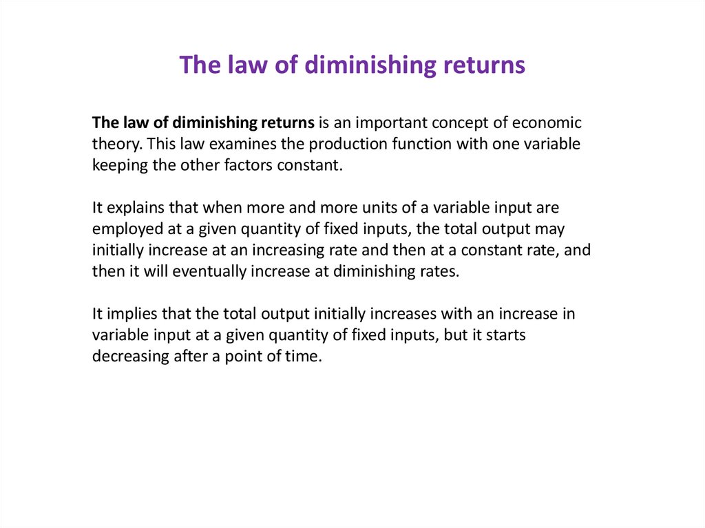
The law of diminishing returns is an important concept of economic
theory. This law examines the production function with one variable
keeping the other factors constant.
It explains that when more and more units of a variable input are
employed at a given quantity of fixed inputs, the total output may
initially increase at an increasing rate and then at a constant rate, and
then it will eventually increase at diminishing rates.
It implies that the total output initially increases with an increase in
variable input at a given quantity of fixed inputs, but it starts
decreasing after a point of time.

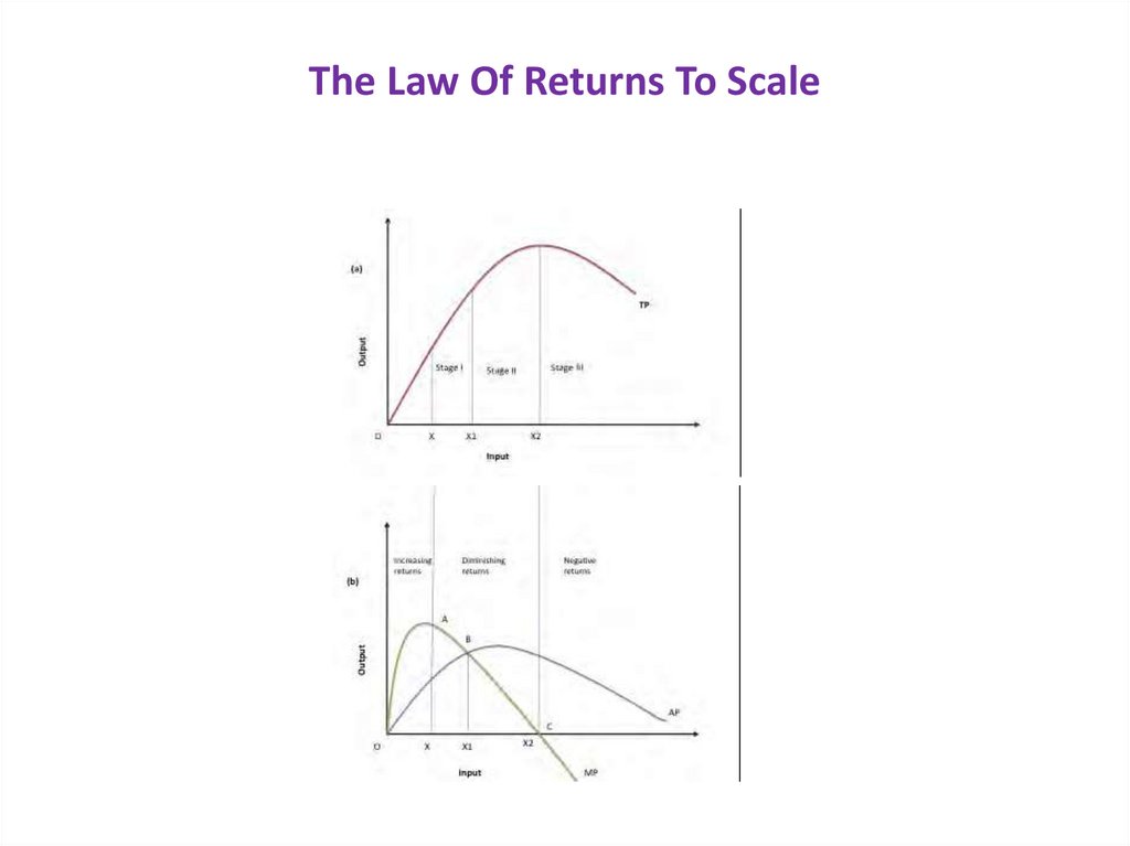
6. The Law Of Returns To Scale

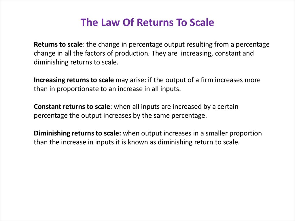
Returns to scale: the change in percentage output resulting from a percentage
change in all the factors of production. They are increasing, constant and
diminishing returns to scale.
Increasing returns to scale may arise: if the output of a firm increases more
than in proportionate to an increase in all inputs.
Constant returns to scale: when all inputs are increased by a certain
percentage the output increases by the same percentage.
Diminishing returns to scale: when output increases in a smaller proportion
than the increase in inputs it is known as diminishing return to scale.

7. The Law Of Returns To Scale

8. ISO-Quants

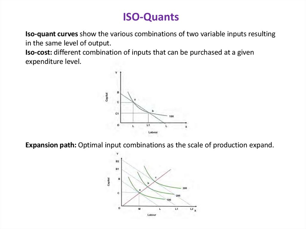
Iso-quant curves show the various combinations of two variable inputs resulting
in the same level of output.
Iso-cost: different combination of inputs that can be purchased at a given
expenditure level.
Expansion path: Optimal input combinations as the scale of production expand.

9. Cost Analysis

The major Cost determinants are:
1.Level of output
2.Price of input factors
3.Productivities of factors of production
4.Size of plant
5.Output stability
6. Lot size
7.Laws of returns
8.Levels of capacity utilization
9.Time period
10.Technology
11.Experience
12.Process of range of products
13.Supply chain and logistics
14.Government incentives

10. Determinants Of Short –Run Cost

Fixed cost: Some inputs are used over a period of time for producing more than
one batch of goods. The costs incurred in these are called fixed cost. For example
amount spent on purchase of equipment, machinery, land and building.
Variable cost: When output has increased the firm spends more on these items.
For example the money spent on labour wages, raw material and electricity usage.
Variable costs vary according to the output. In the long run all costs become
variable.
Total cost: The market value of all resources used to produce a good or service.
Total Fixed cost: Cost of production remains constant whatever the level of
output.
Total Variable cost: Cost of production varies with output.
Average cost: Total cost divided by the level of output.
Average variable cost: Variable cost divided by the level of output.
Average fixed cost: Total fixed cost divided by the level of output.
Marginal cost: Cost of producing an extra unit of output.

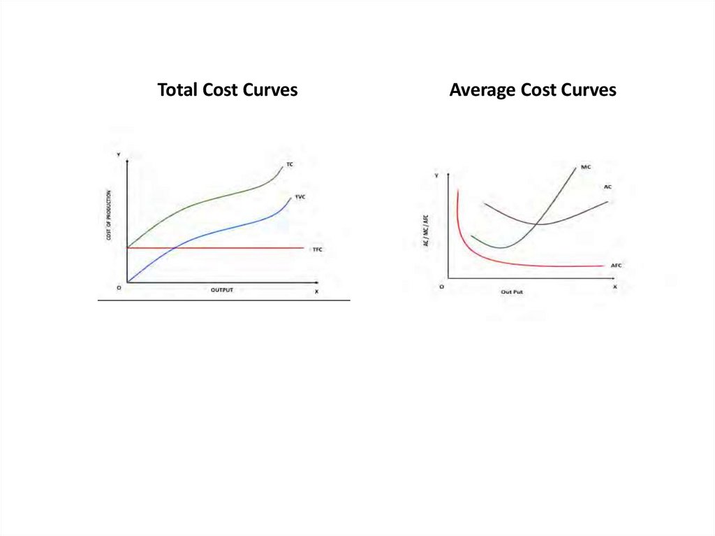
11. Total Cost Curves

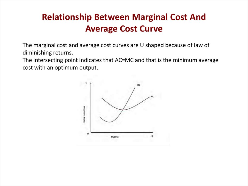
Average Cost Curves

12. Relationship Between Marginal Cost And Average Cost Curve

The marginal cost and average cost curves are U shaped because of law of
diminishing returns.
The intersecting point indicates that AC=MC and that is the minimum average
cost with an optimum output.

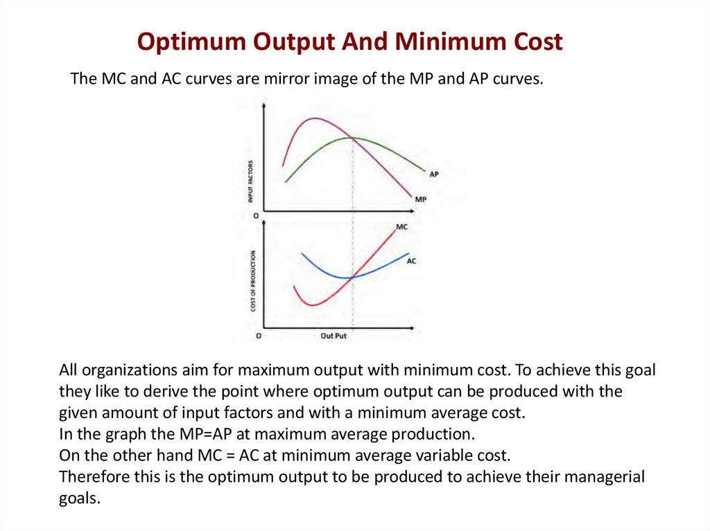
13. Optimum Output And Minimum Cost

The MC and AC curves are mirror image of the MP and AP curves.
All organizations aim for maximum output with minimum cost. To achieve this goal
they like to derive the point where optimum output can be produced with the
given amount of input factors and with a minimum average cost.
In the graph the MP=AP at maximum average production.
On the other hand MC = AC at minimum average variable cost.
Therefore this is the optimum output to be produced to achieve their managerial
goals.

14. Economies Of Scale

Economies of scale exist when long run average costs decline as output is
increased.
Diseconomies of scale exist when long run average cost rises as output is
increased.
The economies of scale occur because of:
1. Technical economies: the change in production process due to technology
adoption
2. Managerial economies
3. Purchasing economies
4. Marketing economies
5. Financial economies.
Economies of scale means a fall in average cost of production due to growth in
the size of the industry within which a firm operates.
Diseconomies of scale arises due to managerial problems. If the size of the
business becomes too large, then it becomes difficult for management to
control the organizational activities therefore diseconomies of scale arise.

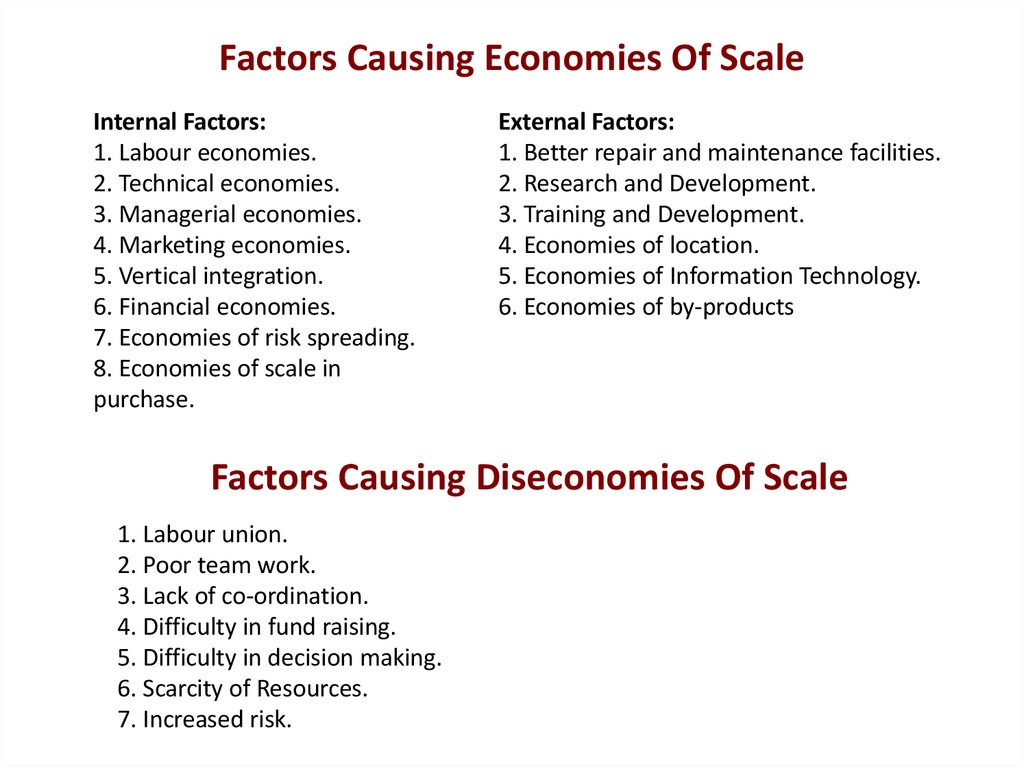
15. Factors Causing Economies Of Scale

Internal Factors:
1. Labour economies.
2. Technical economies.
3. Managerial economies.
4. Marketing economies.
5. Vertical integration.
6. Financial economies.
7. Economies of risk spreading.
8. Economies of scale in
purchase.
External Factors:
1. Better repair and maintenance facilities.
2. Research and Development.
3. Training and Development.
4. Economies of location.
5. Economies of Information Technology.
6. Economies of by-products
Factors Causing Diseconomies Of Scale
1. Labour union.
2. Poor team work.
3. Lack of co-ordination.
4. Difficulty in fund raising.
5. Difficulty in decision making.
6. Scarcity of Resources.
7. Increased risk.

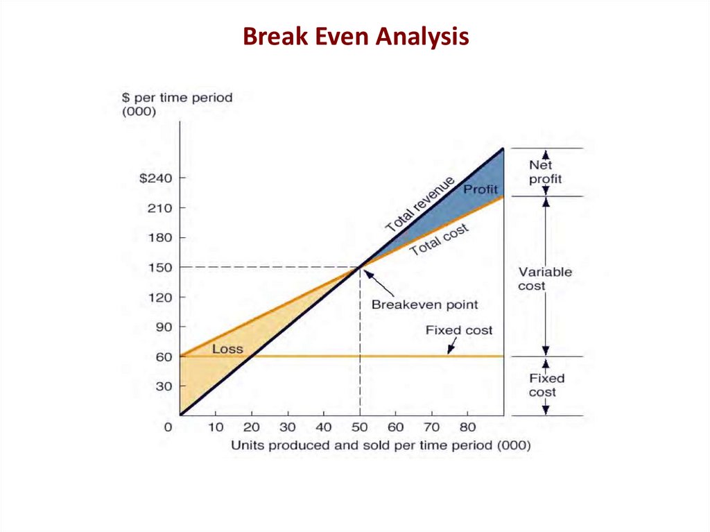
16. Break Even Analysis

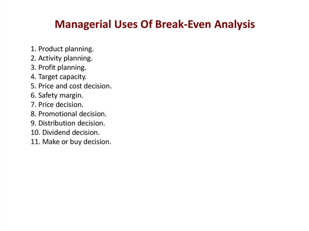
17. Managerial Uses Of Break-Even Analysis

1. Product planning.
2. Activity planning.
3. Profit planning.
4. Target capacity.
5. Price and cost decision.
6. Safety margin.
7. Price decision.
8. Promotional decision.
9. Distribution decision.
10. Dividend decision.
11. Make or buy decision.

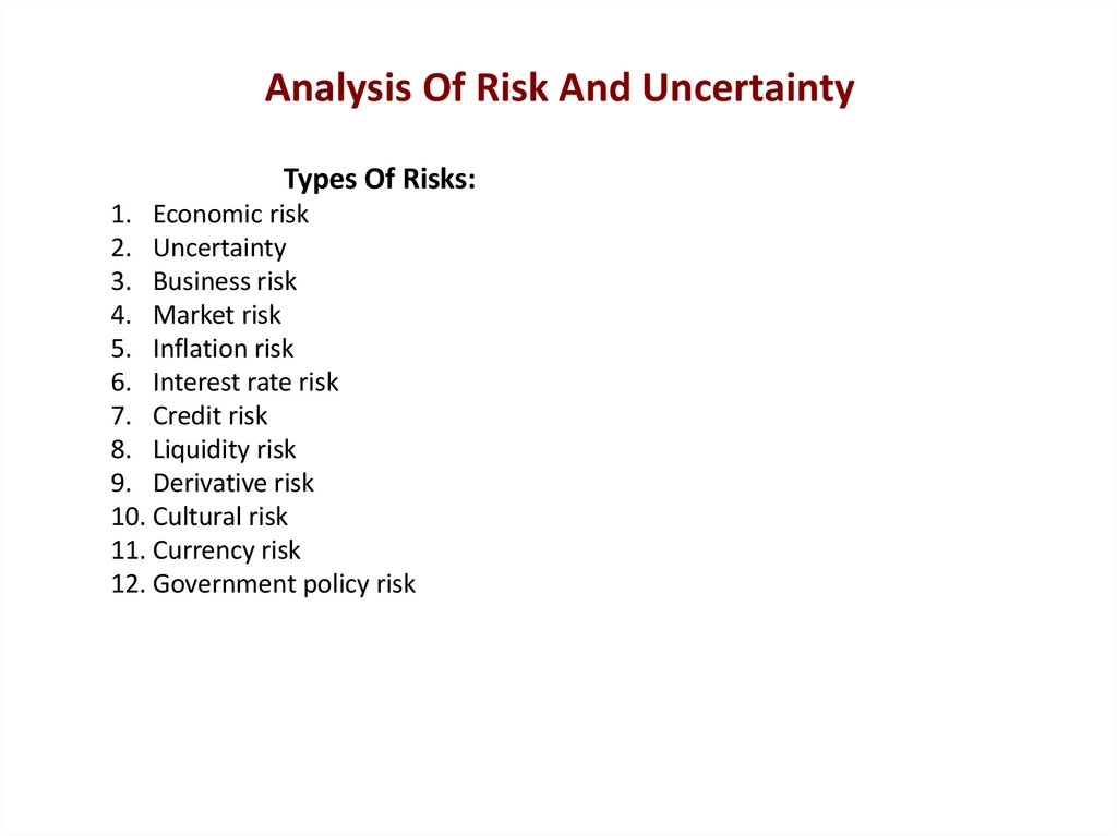
18. Analysis Of Risk And Uncertainty

Types Of Risks:
1. Economic risk
2. Uncertainty
3. Business risk
4. Market risk
5. Inflation risk
6. Interest rate risk
7. Credit risk
8. Liquidity risk
9. Derivative risk
10. Cultural risk
11. Currency risk
12. Government policy risk

19. Probability measurement

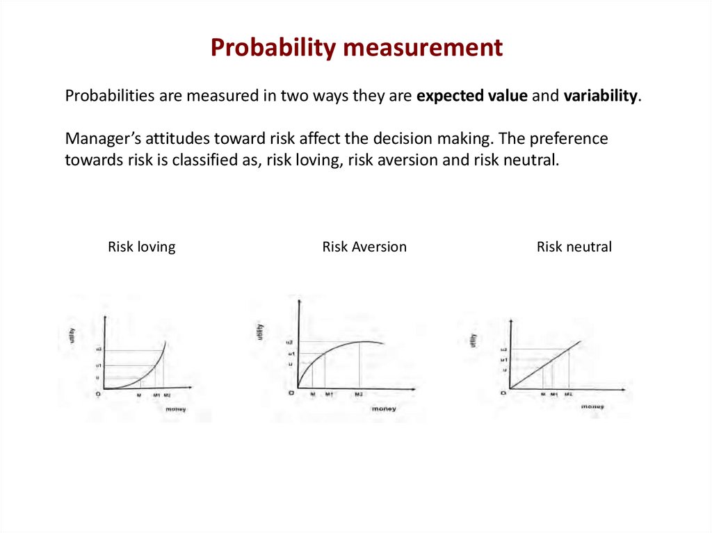
Probabilities are measured in two ways they are expected value and variability.
Manager’s attitudes toward risk affect the decision making. The preference
towards risk is classified as, risk loving, risk aversion and risk neutral.
Risk loving
Risk Aversion
Risk neutral

20. Analysis Of Risk And Uncertainty

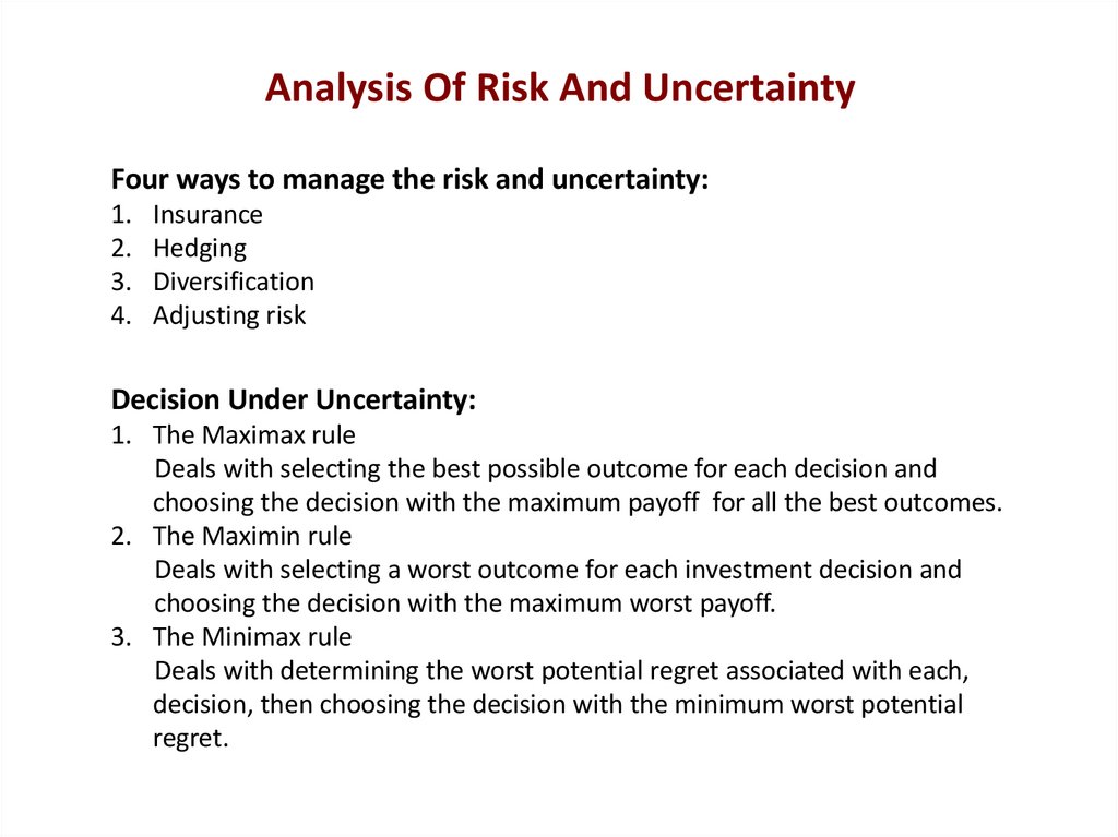
Four ways to manage the risk and uncertainty:
1.
2.
3.
4.
Insurance
Hedging
Diversification
Adjusting risk
Decision Under Uncertainty:
1. The Maximax rule
Deals with selecting the best possible outcome for each decision and
choosing the decision with the maximum payoff for all the best outcomes.
2. The Maximin rule
Deals with selecting a worst outcome for each investment decision and
choosing the decision with the maximum worst payoff.
3. The Minimax rule
Deals with determining the worst potential regret associated with each,
decision, then choosing the decision with the minimum worst potential
regret.