Decision time frames

1. Decision Time Frames

– The firm makes many decisions to achieve its main
objective: profit maximization.
– All decisions can be placed in two time frames:
– The short run
– The long run
1

2. Decision Time Frames

• The Short Run
– The short run is a time frame in which the quantity of
one or more resources used in production is fixed.
– For most firms, the capital, called the firm’s plant, is
fixed in the short run.
– Other resources used by the firm (such as labor, raw
materials, and energy) can be changed in the short run.
– Short-run decisions are easily reversed.
2

3. Decision Time Frames

• The Long Run
– The long run is a time frame in which the quantities of
all resources—including the plant size—can be varied.
– Long-run decisions are not easily reversed.
– A sunk cost is a cost incurred by the firm and cannot
be changed.
– If a firm’s plant has no resale value, the amount paid for
it is a sunk cost.
– Sunk costs are irrelevant to a firm’s decisions.
3

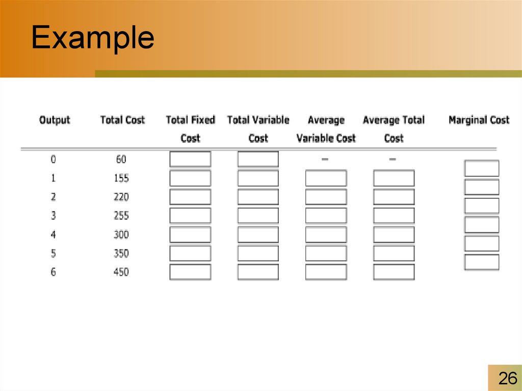
4. Example

With regard to economic decision making for
firms, the short run is
– A) a definite number of months.
– B) a period over which the quantities of all factors of
production and technology are variable.
– C) a period over which the quantity of at least one
significant factor of production is fixed.
– D) a period over which the quantities of all factors of
production are variable but technology is fixed.
– E) less than one year.
4

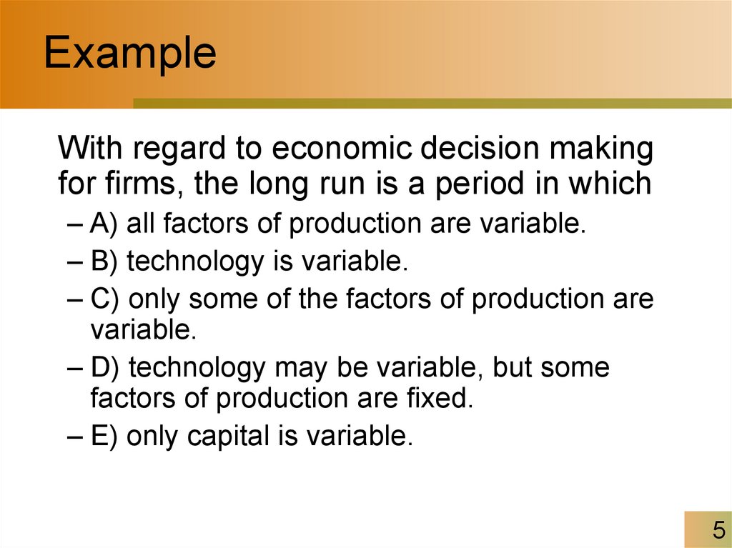
5. Example

With regard to economic decision making
for firms, the long run is a period in which
– A) all factors of production are variable.
– B) technology is variable.
– C) only some of the factors of production are
variable.
– D) technology may be variable, but some
factors of production are fixed.
– E) only capital is variable.
5

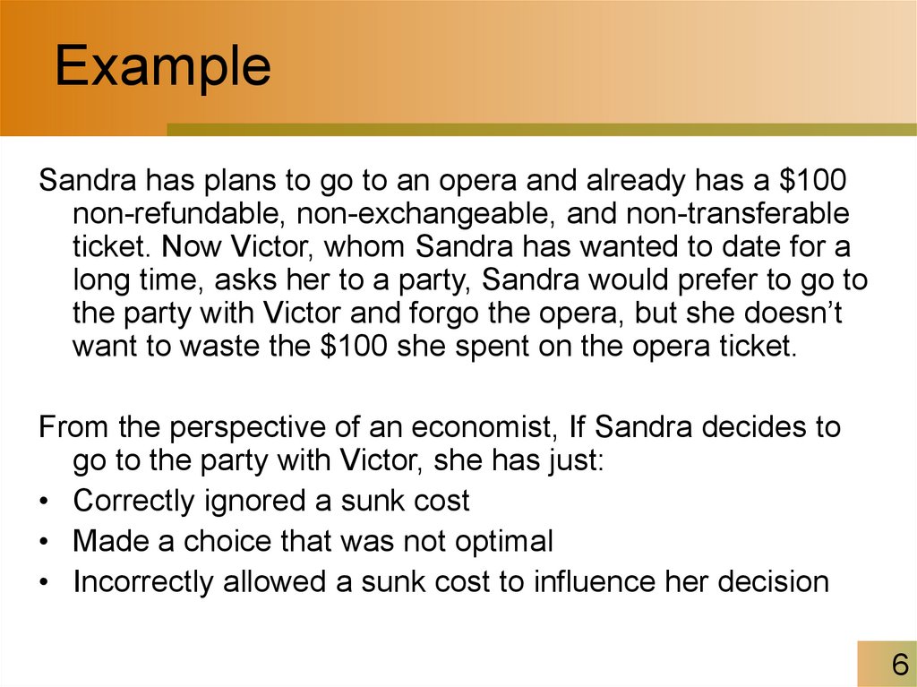
6. Example

Sandra has plans to go to an opera and already has a $100
non-refundable, non-exchangeable, and non-transferable
ticket. Now Victor, whom Sandra has wanted to date for a
long time, asks her to a party, Sandra would prefer to go to
the party with Victor and forgo the opera, but she doesn’t
want to waste the $100 she spent on the opera ticket.
From the perspective of an economist, If Sandra decides to
go to the party with Victor, she has just:
• Correctly ignored a sunk cost
• Made a choice that was not optimal
• Incorrectly allowed a sunk cost to influence her decision
6

7. Short-Run Technology Constraint

– To increase output in the short run, a firm must increase
the amount of labor employed.
– Three concepts describe the relationship between
output and the quantity of labor employed:
• Total product
• Marginal product
• Average product
7

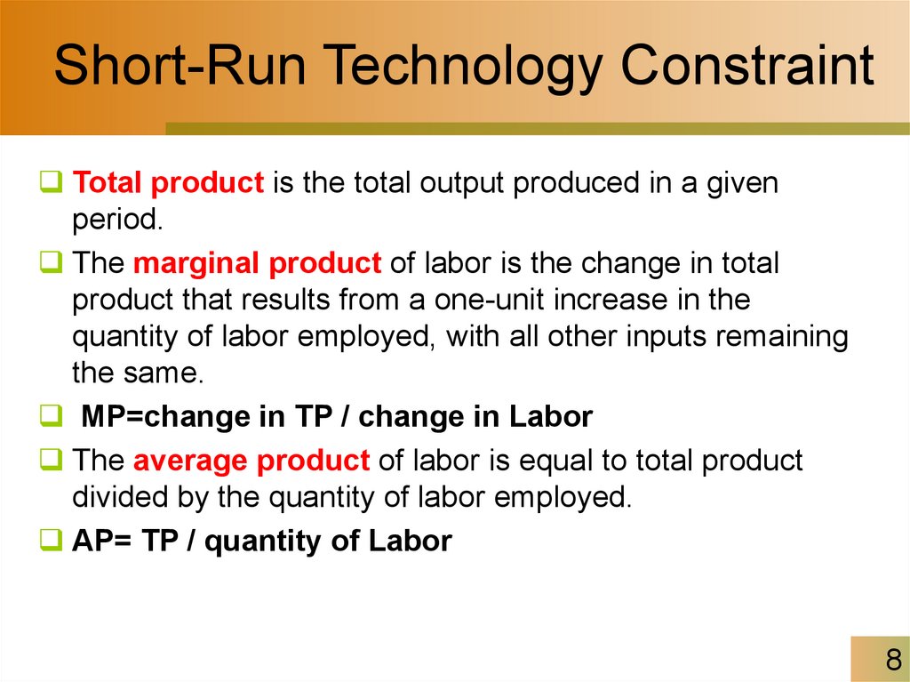
8. Short-Run Technology Constraint

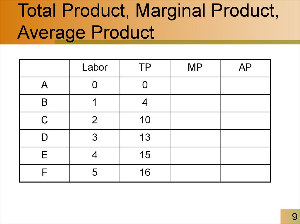
Total product is the total output produced in a given
period.
The marginal product of labor is the change in total
product that results from a one-unit increase in the
quantity of labor employed, with all other inputs remaining
the same.
MP=change in TP / change in Labor
The average product of labor is equal to total product
divided by the quantity of labor employed.
AP= TP / quantity of Labor
8

9. Total Product, Marginal Product, Average Product

Labor
TP
A
0
0
B
1
4
C
2
10
D
3
13
E
4
15
F
5
16
MP
AP
9

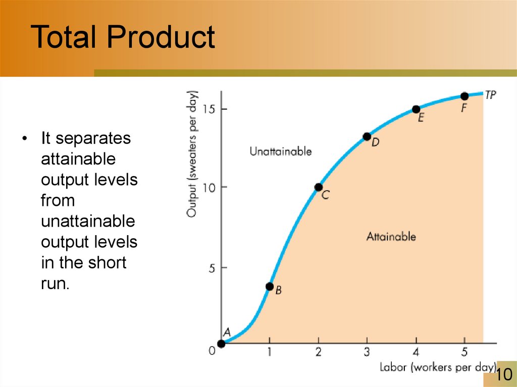
10. Total Product

• It separates
attainable
output levels
from
unattainable
output levels
in the short
run.
10

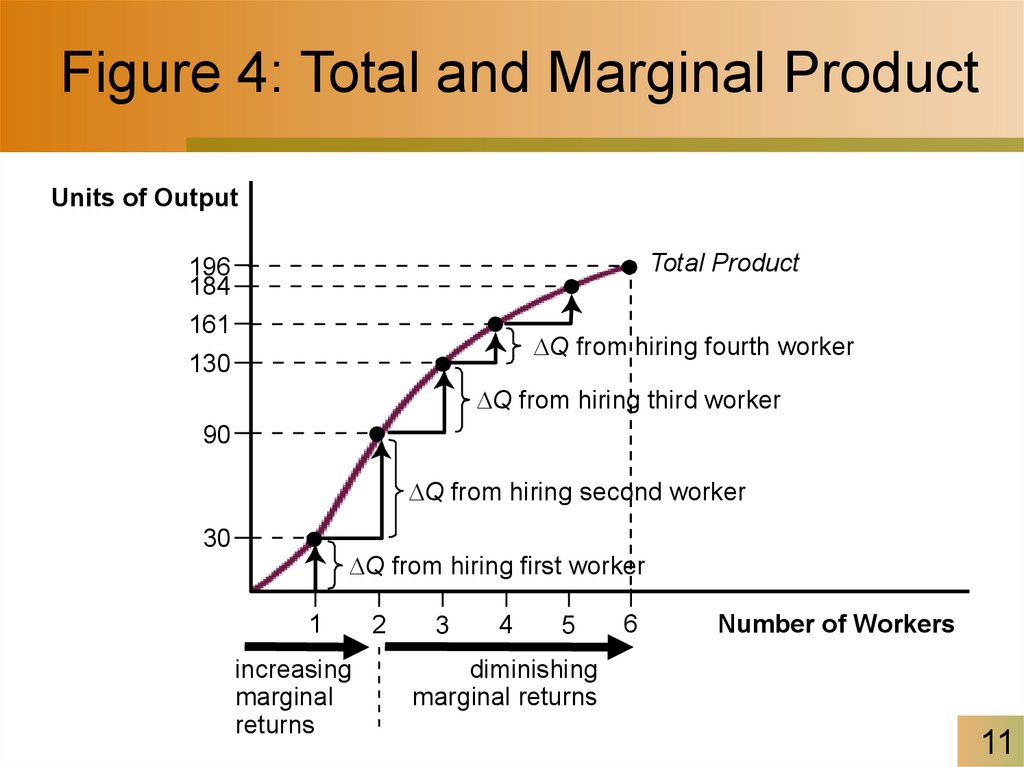
11. Figure 4: Total and Marginal Product

Units of Output
Total Product
196
184
161
DQ from hiring fourth worker
130
DQ from hiring third worker
90
DQ from hiring second worker
30
DQ from hiring first worker
1
increasing
marginal
returns
2
3
4
5
6
Number of Workers
diminishing
marginal returns
11

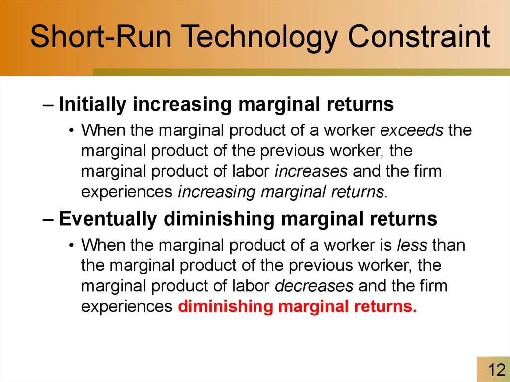
12. Short-Run Technology Constraint

– Initially increasing marginal returns
• When the marginal product of a worker exceeds the
marginal product of the previous worker, the
marginal product of labor increases and the firm
experiences increasing marginal returns.
– Eventually diminishing marginal returns
• When the marginal product of a worker is less than
the marginal product of the previous worker, the
marginal product of labor decreases and the firm
experiences diminishing marginal returns.
12

13. Short-Run Technology Constraint

• Increasing marginal returns arise from increased
specialization and division of labor.
• Diminishing marginal returns arises from the fact that
employing additional units of labor means each worker
has less access to capital and less space in which to
work.
• The law of diminishing returns states that as a firm
uses more of a variable input with a given quantity of
fixed inputs, the marginal product of the variable input
eventually diminishes.
13

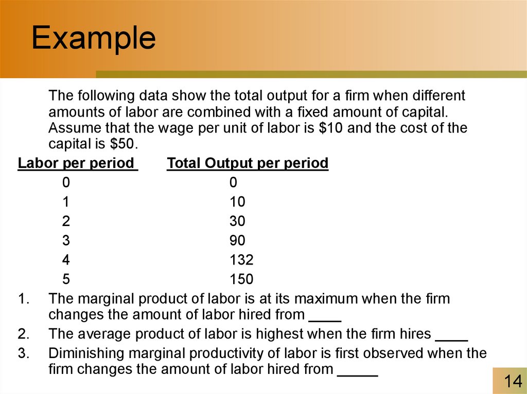
14. Example

The following data show the total output for a firm when different
amounts of labor are combined with a fixed amount of capital.
Assume that the wage per unit of labor is $10 and the cost of the
capital is $50.
Labor per period
Total Output per period
0
0
1
10
2
30
3
90
4
132
5
150
1. The marginal product of labor is at its maximum when the firm
changes the amount of labor hired from ____
2. The average product of labor is highest when the firm hires ____
3. Diminishing marginal productivity of labor is first observed when the
firm changes the amount of labor hired from _____
14

15. Short-Run Technology Constraint

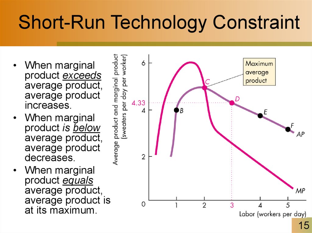
• When marginal
product exceeds
average product,
average product
increases.
• When marginal
product is below
average product,
average product
decreases.
• When marginal
product equals
average product,
average product is
at its maximum.
15

16. Example

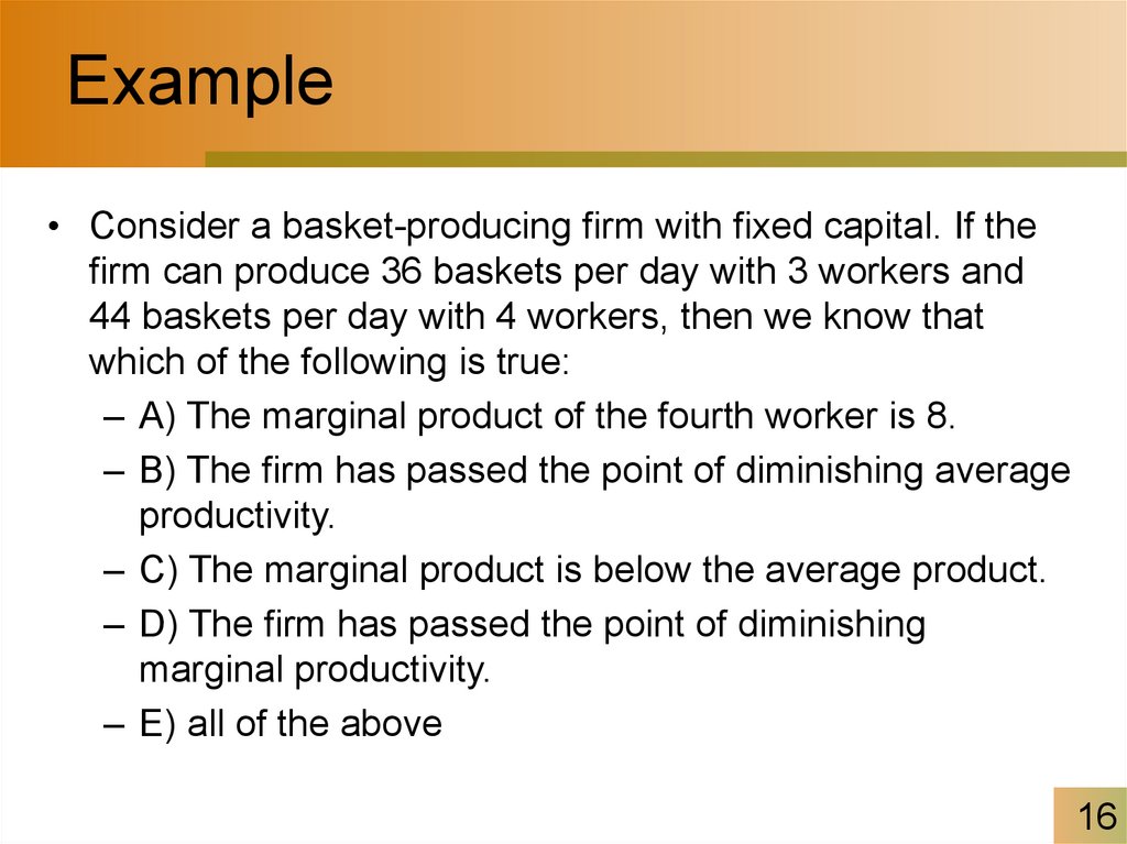
• Consider a basket-producing firm with fixed capital. If the
firm can produce 36 baskets per day with 3 workers and
44 baskets per day with 4 workers, then we know that
which of the following is true:
– A) The marginal product of the fourth worker is 8.
– B) The firm has passed the point of diminishing average
productivity.
– C) The marginal product is below the average product.
– D) The firm has passed the point of diminishing
marginal productivity.
– E) all of the above
16

17. Short-Run Cost

– To produce more output in the short run, the firm must
employ more labor, which means that it must increase
its costs.
– We describe the way a firm’s costs change as total
product changes by using three cost concepts and
three types of cost curve:
• Total cost
• Marginal cost
• Average cost
17

18. Short-Run Cost

• Total Cost
– A firm’s total cost (TC) is the cost of all resources
used.
– Total fixed cost (TFC) is the cost of the firm’s fixed
inputs. Fixed costs do not change with output.
– Total variable cost (TVC) is the cost of the firm’s
variable inputs. Variable costs do change with output.
– Total cost equals total fixed cost plus total variable cost.
That is:
TC = TFC + TVC
18

19. Total Costs of Production

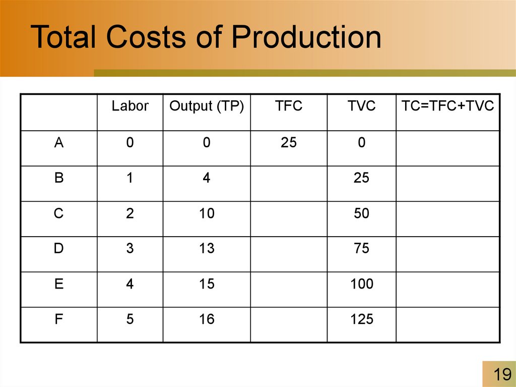
Labor
Output (TP)
TFC
TVC
A
0
0
25
0
B
1
4
25
C
2
10
50
D
3
13
75
E
4
15
100
F
5
16
125
TC=TFC+TVC
19

20. Example

Larry’s Performance Pizza is a small restaurant that sells
low-carbohydrate pizzas in a health - conscious town.
Larry’s very tiny kitchen has enough room for the 4 ovens
in which his workers bake the pizzas. Larry signed a lease
obligating him to pay the rent for the four ovens for the
next year. Because of this, and because Larry’s kitchen
cannot fit more than four ovens, Larry cannot change the
number of ovens he uses in his production of pizzas in the
short run.
On the other hand, Larry’s workers tend to be students. Each
Monday, Larry lets them know how many hours he’ll need
them for that week. In the short run, these workers are
______ inputs, and the ovens are _______ inputs.
20

21. Total Costs of Production

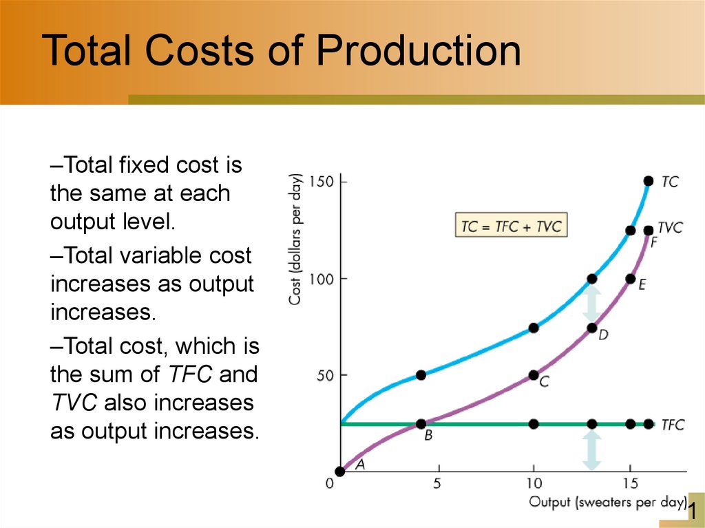
–Total fixed cost is
the same at each
output level.
–Total variable cost
increases as output
increases.
–Total cost, which is
the sum of TFC and
TVC also increases
as output increases.
21

22. Short-Run Cost

• Marginal Cost
– Marginal cost (MC) is the increase in total cost that
results from a one-unit increase in total product.
– Over the output range with increasing marginal returns,
marginal cost falls as output increases.
– Over the output range with diminishing marginal
returns, marginal cost rises as output increases.
22

23. Short-Run Cost

• Average Cost
– Average cost measures can be derived from each of
the total cost measures:
– Average fixed cost (AFC) is total fixed cost per unit of
output.
– Average variable cost (AVC) is total variable cost per
unit of output.
– Average total cost (ATC) is total cost per unit of
output.
ATC = AFC + AVC.
23

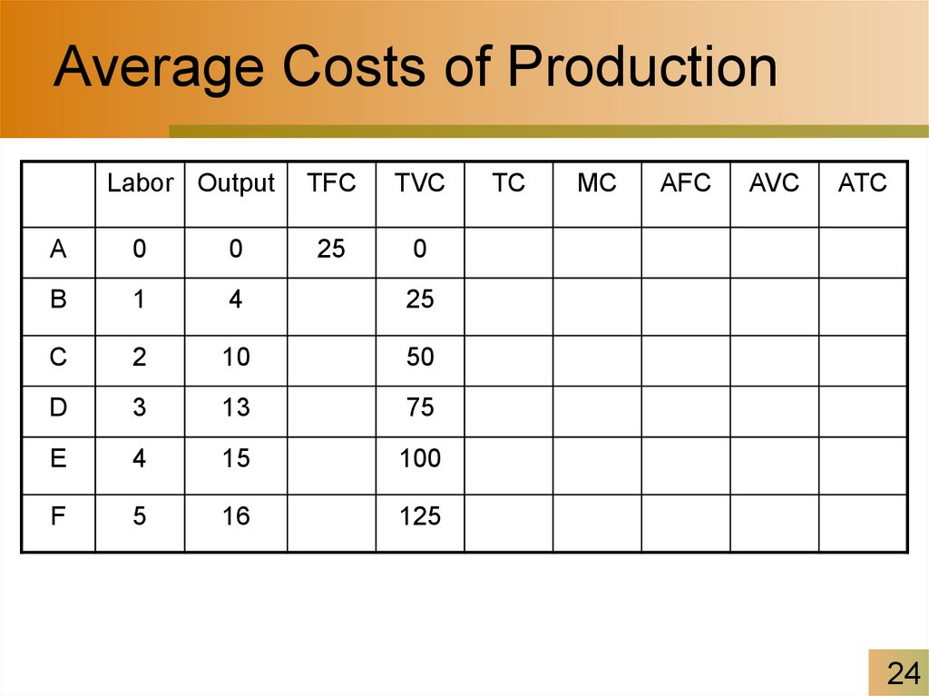
24. Average Costs of Production

Labor Output
TFC
TVC
25
0
A
0
0
B
1
4
25
C
2
10
50
D
3
13
75
E
4
15
100
F
5
16
125
TC
MC
AFC
AVC
ATC
24

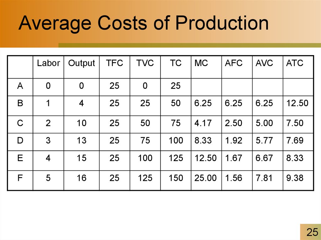
25. Average Costs of Production

Labor Output
TFC
TVC
TC
MC
AFC
AVC
ATC
A
0
0
25
0
25
B
1
4
25
25
50
6.25
6.25
6.25
12.50
C
2
10
25
50
75
4.17
2.50
5.00
7.50
D
3
13
25
75
100
8.33
1.92
5.77
7.69
E
4
15
25
100
125
12.50 1.67
6.67
8.33
F
5
16
25
125
150
25.00 1.56
7.81
9.38
25

26. Example

26

27. Example

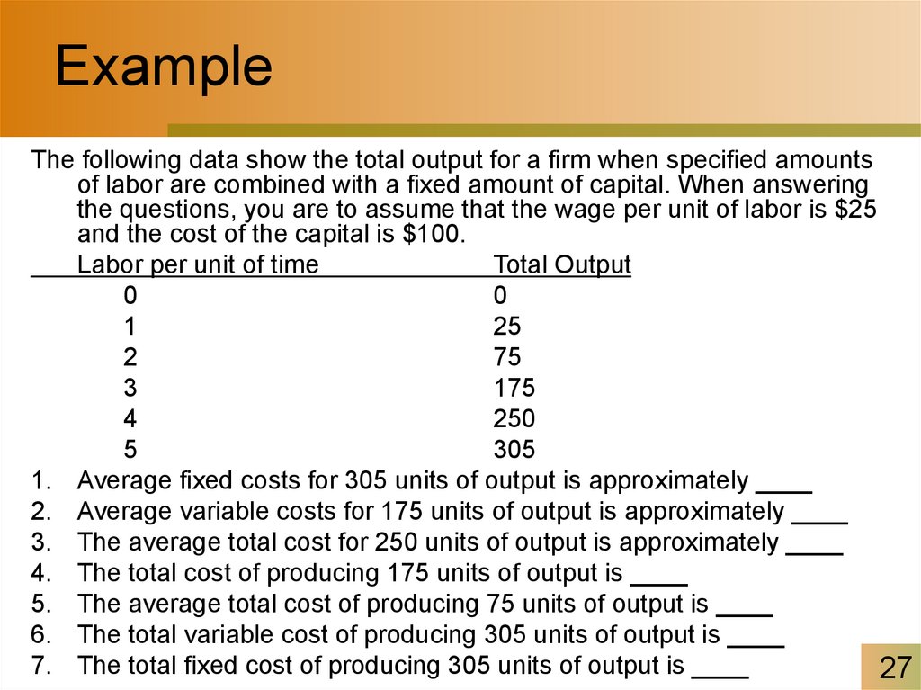
The following data show the total output for a firm when specified amounts
of labor are combined with a fixed amount of capital. When answering
the questions, you are to assume that the wage per unit of labor is $25
and the cost of the capital is $100.
Labor per unit of time
Total Output
0
0
1
25
2
75
3
175
4
250
5
305
1. Average fixed costs for 305 units of output is approximately ____
2. Average variable costs for 175 units of output is approximately ____
3. The average total cost for 250 units of output is approximately ____
4. The total cost of producing 175 units of output is ____
5. The average total cost of producing 75 units of output is ____
6. The total variable cost of producing 305 units of output is ____
7. The total fixed cost of producing 305 units of output is ____
27

28. Average And Marginal Costs

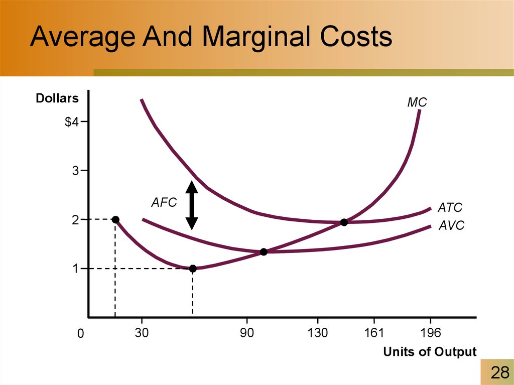
Dollars
MC
$4
3
AFC
ATC
AVC
2
1
0
30
90
130
161
196
Units of Output
28

29. The Relationship Between Average And Marginal Costs

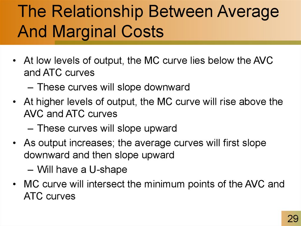
• At low levels of output, the MC curve lies below the AVC
and ATC curves
– These curves will slope downward
• At higher levels of output, the MC curve will rise above the
AVC and ATC curves
– These curves will slope upward
• As output increases; the average curves will first slope
downward and then slope upward
– Will have a U-shape
• MC curve will intersect the minimum points of the AVC and
ATC curves
29

30. Example

Suppose a firm producing digital cameras is operating such
that marginal costs are higher than average costs. If the firm
produces one more camera, average costs will
– A) rise.
– B) fall.
– C) reach a point of diminishing returns.
– D) remain constant.
– E) reach their maximum.
30

31. Short-Run Cost

• Shifts in Cost Curves
The position of a firm’s cost curves depend on
two factors:
– Technology
– Prices of productive resources
31

32. Short-Run Cost

Technological change influences both the
productivity curves and the cost curves.
– An increase in productivity shifts the average and
marginal product curves upward and the average and
marginal cost curves downward.
– If a technological advance brings more capital and less
labor into use, fixed costs increase and variable costs
decrease.
– In this case, average total cost increases at low output
levels and decreases at high output levels.
32

33. Short-Run Cost

• Changes in the prices of resources shift the cost
curves.
– An increase in a fixed cost shifts the total cost (TC ) and
average total cost (ATC) curves upward but does not
shift the marginal cost (MC) curve.
– An increase in a variable cost shifts the total cost (TC),
average total cost (ATC), and marginal cost (MC)
curves upward.
33

34. Example

• In the short run, when capital is a fixed factor, a rise in the
cost of labor
– A) shifts the marginal cost curve upwards.
– B) shifts the AVC curve down.
– C) shifts the total product curve downwards.
– D) leaves the MC curve unchanged.
– E) leaves the ATC curve unchanged.
34

35. Production And Cost in the Long Run

• In the long run, costs behave differently
– Firm can adjust all of its inputs in any way it wants
• In the long run, there are no fixed inputs or fixed
costs
• The firm’s goal is to earn the highest possible
profit
– To do this, it must follow the least cost rule
• To produce any given level of output the firm will
choose the input mix with the lowest cost
35

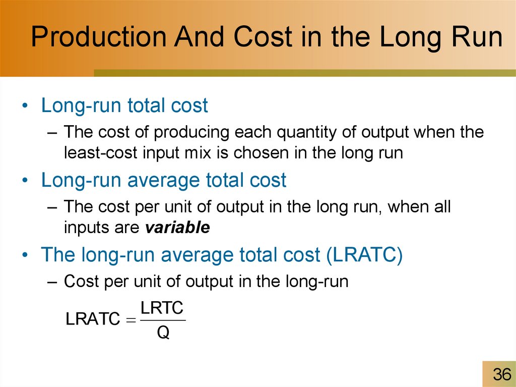
36. Production And Cost in the Long Run

• Long-run total cost
– The cost of producing each quantity of output when the
least-cost input mix is chosen in the long run
• Long-run average total cost
– The cost per unit of output in the long run, when all
inputs are variable
• The long-run average total cost (LRATC)
– Cost per unit of output in the long-run
LRTC
LRATC
Q
36

37. Long-Run Cost

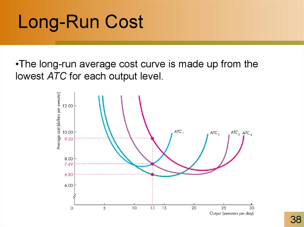
• The average cost of producing a given output varies and
depends on the firm’s plant size.
• The larger the plant size, the greater is the output at which
ATC is at a minimum.
• Cindy has 4 different plant sizes: 1, 2, 3, or 4 knitting
machines.
• Each plant has a short-run ATC curve.
• The firm can compare the ATC for each given output at
different plant sizes.
37

38. Long-Run Cost

•The long-run average cost curve is made up from the
lowest ATC for each output level.
38

39. Long-Run Cost

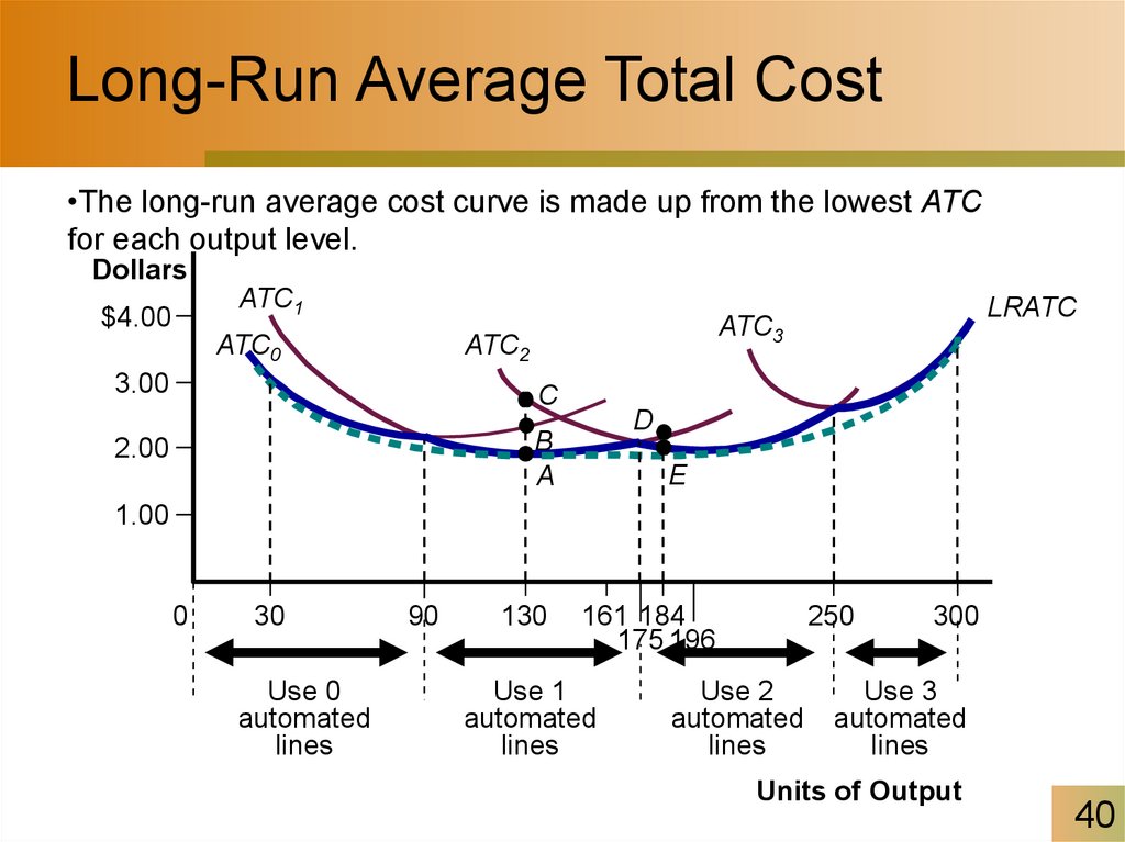
• Long-Run Average Cost Curve
– The long-run average cost curve is the relationship
between the lowest attainable average total cost and
output when both the plant size and labor are varied.
– The long-run average cost curve is a planning curve
that tells the firm the plant size that minimizes the cost
of producing a given output range.
– Once the firm has chosen that plant size, it incurs the
costs that correspond to the ATC curve for that plant.
39

40. Long-Run Average Total Cost

•The long-run average cost curve is made up from the lowest ATC
for each output level.
Dollars
ATC1
$4.00
ATC0
ATC2
3.00
C
D
B
A
2.00
LRATC
ATC3
E
1.00
0
30
Use 0
automated
lines
90
130
161 184
175 196
Use 1
automated
lines
250
Use 2
automated
lines
300
Use 3
automated
lines
Units of Output
40

41. Example

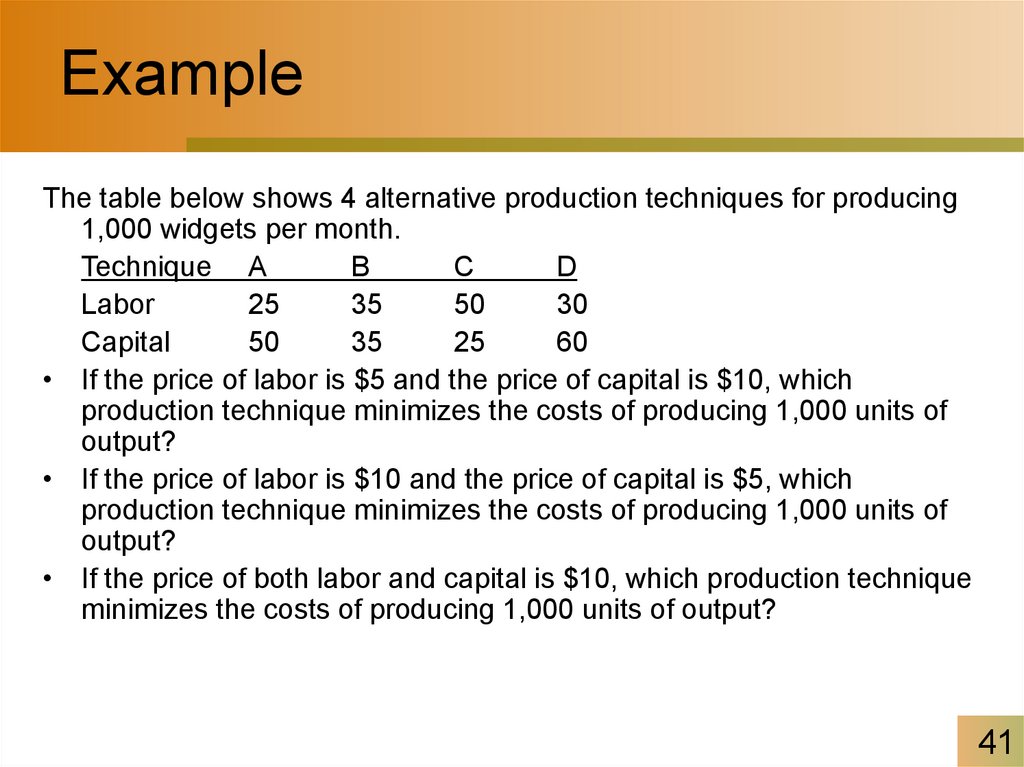
The table below shows 4 alternative production techniques for producing
1,000 widgets per month.
Technique A
B
C
D
Labor
25
35
50
30
Capital
50
35
25
60
• If the price of labor is $5 and the price of capital is $10, which
production technique minimizes the costs of producing 1,000 units of
output?
• If the price of labor is $10 and the price of capital is $5, which
production technique minimizes the costs of producing 1,000 units of
output?
• If the price of both labor and capital is $10, which production technique
minimizes the costs of producing 1,000 units of output?
41

42. Example

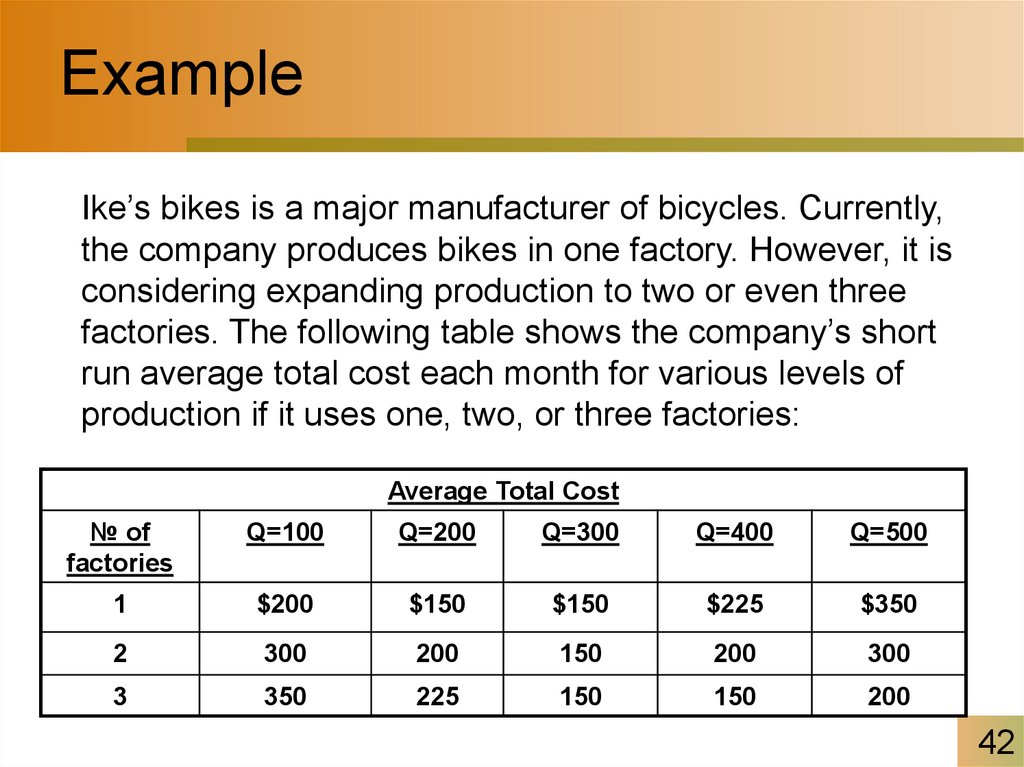
Ike’s bikes is a major manufacturer of bicycles. Currently,
the company produces bikes in one factory. However, it is
considering expanding production to two or even three
factories. The following table shows the company’s short
run average total cost each month for various levels of
production if it uses one, two, or three factories:
Average Total Cost
№ of
factories
Q=100
Q=200
Q=300
Q=400
Q=500
1
$200
$150
$150
$225
$350
2
300
200
150
200
300
3
350
225
150
150
200
42

43. Example

Average Total Cost
№ of
factories
Q=100
Q=200
Q=300
Q=400
Q=500
1
$200
$150
$150
$225
$350
2
300
200
150
200
300
3
350
225
150
150
200
1. Suppose Ike’s Bikes is currently producing 500 bikes per month
in its (only) factory. Its short-run average total cost is ____ per
bike.
2. Suppose Ike’s Bikes is expected to produce 500 bikes per
month for several years. In this case, in the long run, it would
choose to produce bikes using ______.
43

44. Long-Run Cost

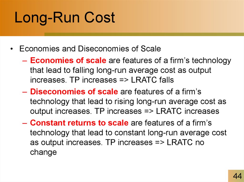
• Economies and Diseconomies of Scale
– Economies of scale are features of a firm’s technology
that lead to falling long-run average cost as output
increases. TP increases => LRATC falls
– Diseconomies of scale are features of a firm’s
technology that lead to rising long-run average cost as
output increases. TP increases => LRATC increases
– Constant returns to scale are features of a firm’s
technology that lead to constant long-run average cost
as output increases. TP increases => LRATC no
change
44

45. The Shape Of LRATC

Dollars
$4.00
3.00
LRATC
2.00
1.00
130
0
Economies of Scale
184
Constant
Returns to
Scale
Diseconomies of Scale
Units of Output
45

46. Example

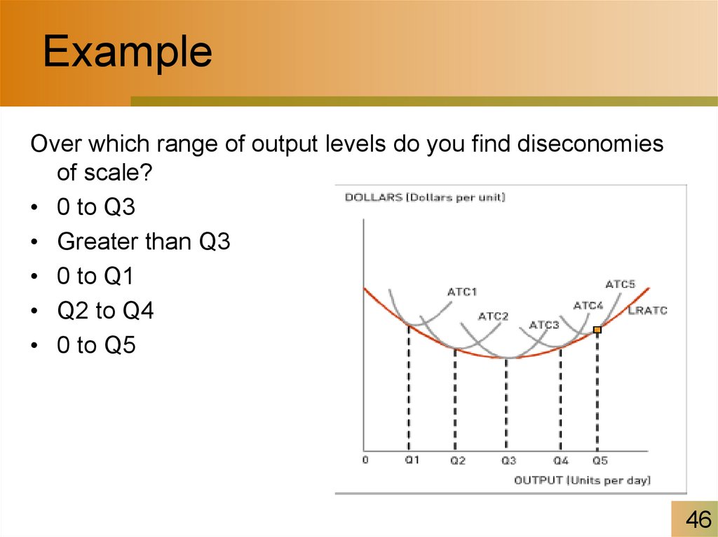
Over which range of output levels do you find diseconomies
of scale?
• 0 to Q3
• Greater than Q3
• 0 to Q1
• Q2 to Q4
• 0 to Q5
46

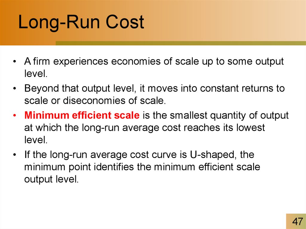
47. Long-Run Cost

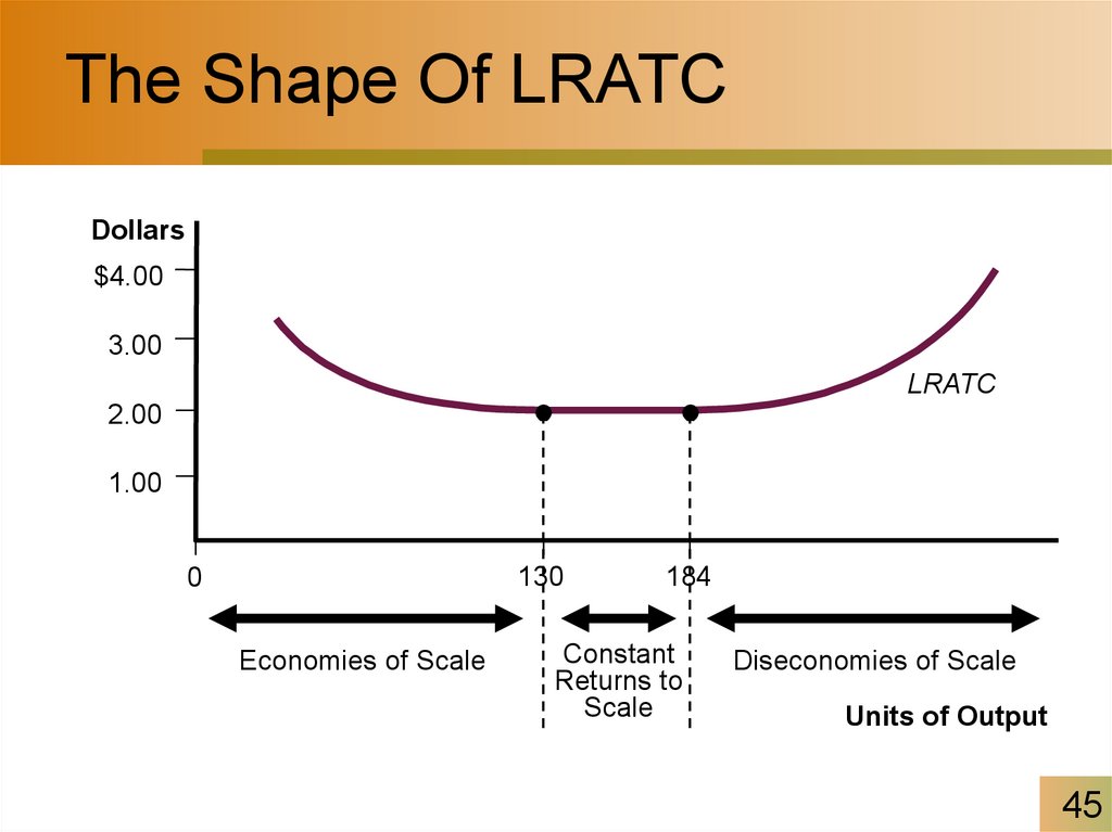
• A firm experiences economies of scale up to some output
level.
• Beyond that output level, it moves into constant returns to
scale or diseconomies of scale.
• Minimum efficient scale is the smallest quantity of output
at which the long-run average cost reaches its lowest
level.
• If the long-run average cost curve is U-shaped, the
minimum point identifies the minimum efficient scale
output level.
47

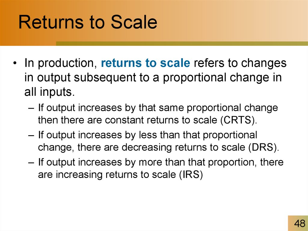
48. Returns to Scale

• In production, returns to scale refers to changes
in output subsequent to a proportional change in
all inputs.
– If output increases by that same proportional change
then there are constant returns to scale (CRTS).
– If output increases by less than that proportional
change, there are decreasing returns to scale (DRS).
– If output increases by more than that proportion, there
are increasing returns to scale (IRS)
48

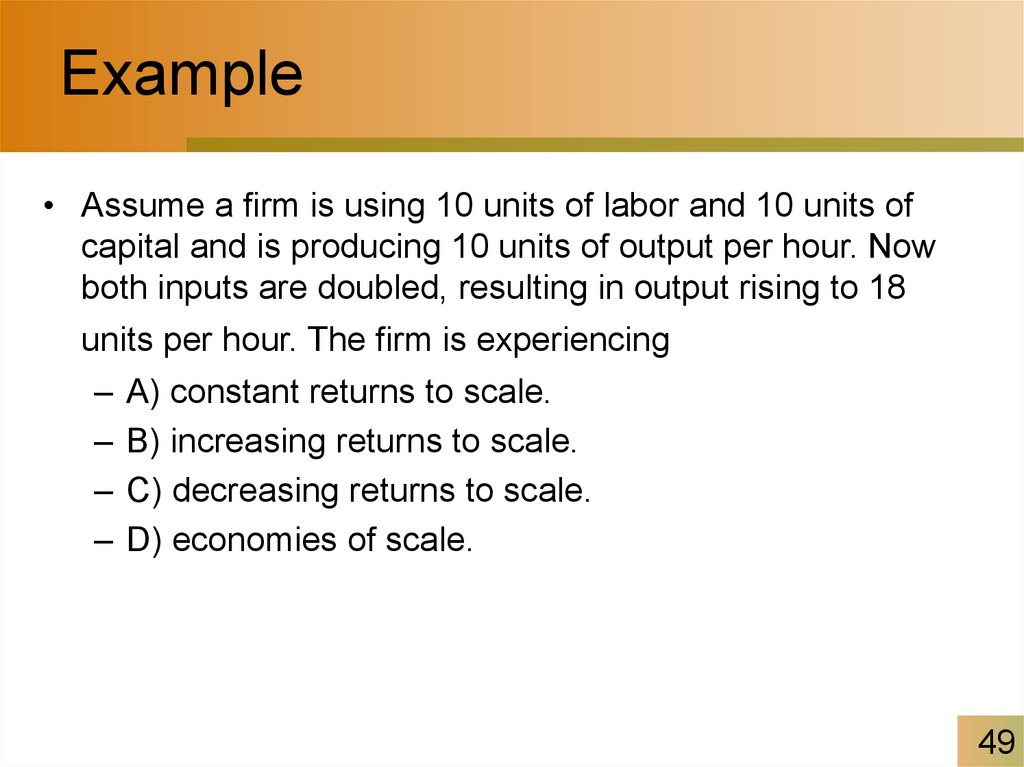
49. Example

• Assume a firm is using 10 units of labor and 10 units of
capital and is producing 10 units of output per hour. Now
both inputs are doubled, resulting in output rising to 18
units per hour. The firm is experiencing
–
–
–
–
A) constant returns to scale.
B) increasing returns to scale.
C) decreasing returns to scale.
D) economies of scale.
49

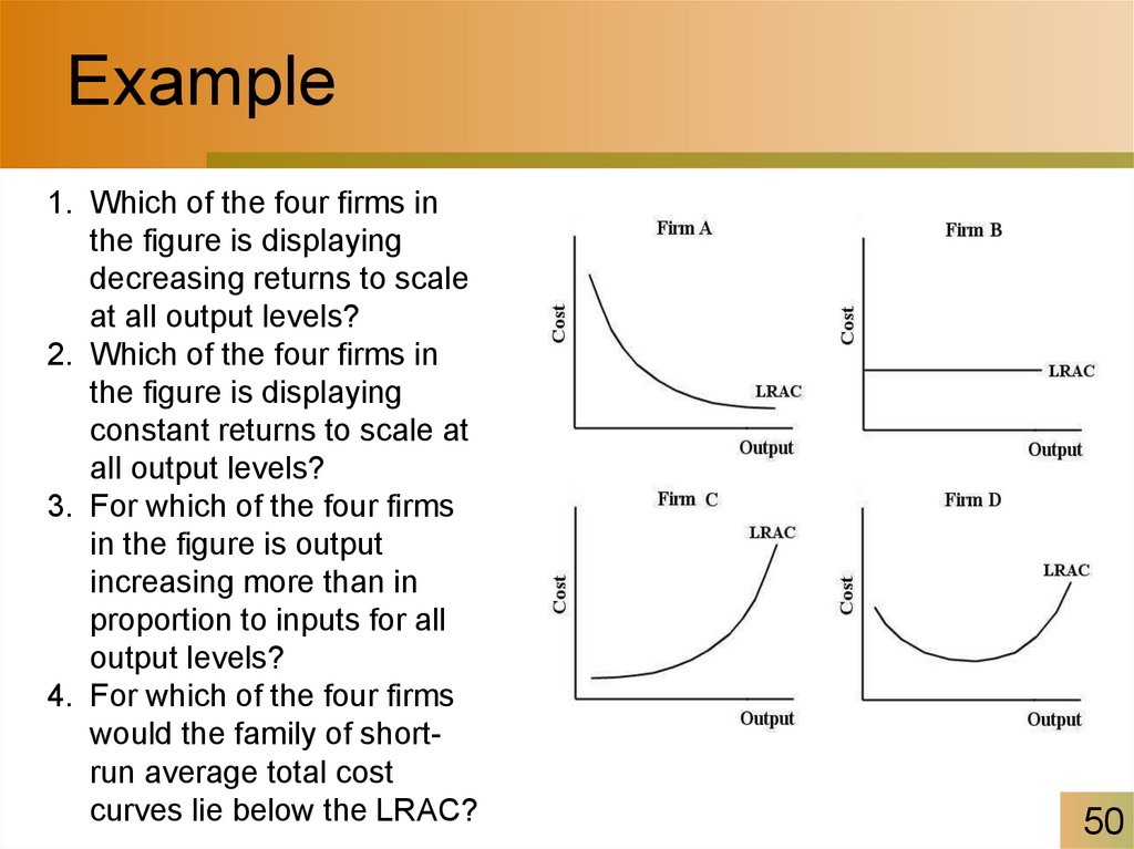
50. Example

1. Which of the four firms in
the figure is displaying
decreasing returns to scale
at all output levels?
2. Which of the four firms in
the figure is displaying
constant returns to scale at
all output levels?
3. For which of the four firms
in the figure is output
increasing more than in
proportion to inputs for all
output levels?
4. For which of the four firms
would the family of shortrun average total cost
curves lie below the LRAC?
50