Management Science

1. Management Science

Chapter 1
Copyright © 2010 Pearson Education, Inc. Publishing as Prentice Hall
1-1

2. BA 250 Management Science

Management
science,
also
known
as
Operations Research, Quantitative Methods,
etc.,
involves a logical mathematical
approach to problem solving.
- used in a variety of organizations to
solve many different types of problems in
manufacturing, marketing, finance, logistics.
Copyright © 2010 Pearson Education, Inc. Publishing as Prentice Hall
1-2

3. Text Book

Introduction to Management Science
Bernard W. Taylor III,
12th Edition, Prentice Hall, New Jersey
Copyright © 2010 Pearson Education, Inc. Publishing as Prentice Hall
1-3

4. Learning Outcomes

The students who succeed in this course;
define basic mathematical modeling concepts and
techniques
formulate a variety of management problems in
marketing, production, logistics and finance
apply basic mathematical optimization models
including
linear
programming
and
integer
programming
interpret the computer output generated from “QM for
Windows” to solve linear programming models
analyze various decision making problems under
certainty, uncertainty and risk
Copyright © 2010 Pearson Education, Inc. Publishing as Prentice Hall
1-4

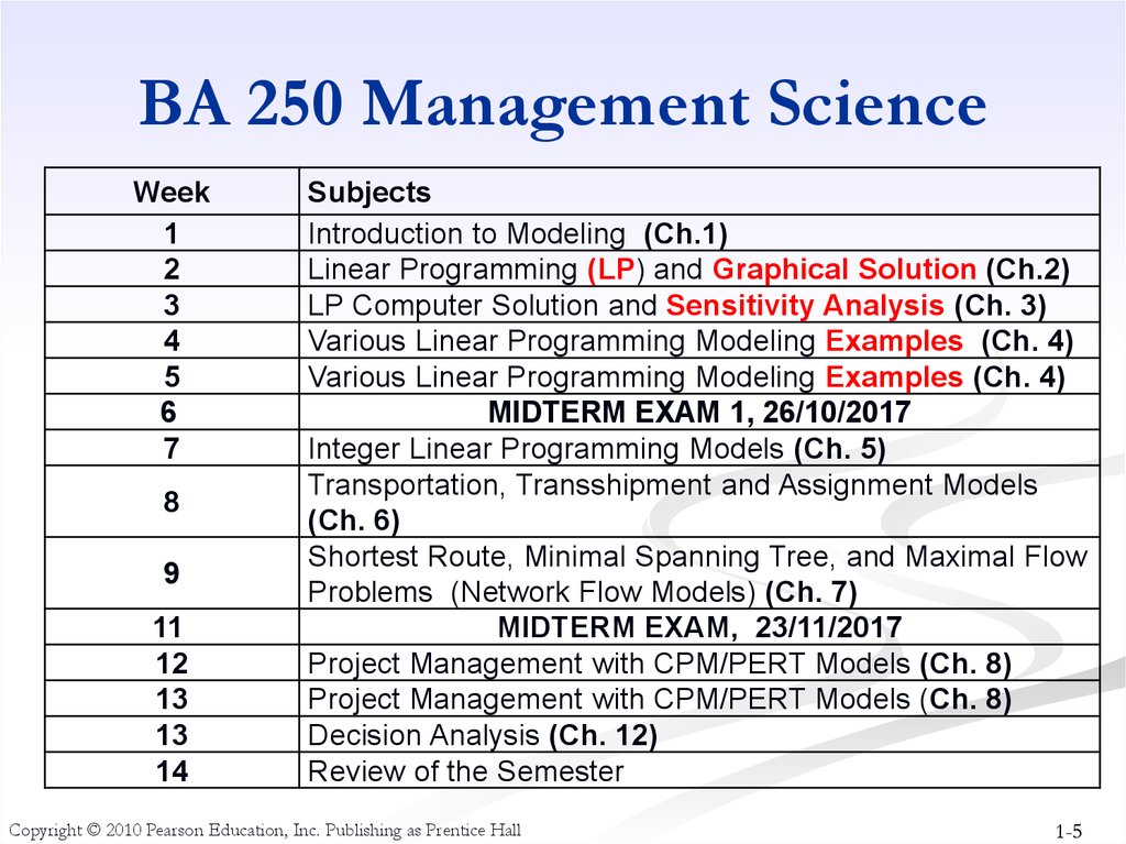
5. BA 250 Management Science

Week
1
2
3
4
5
6
7
8
9
11
12
13
13
14
Subjects
Introduction to Modeling (Ch.1)
Linear Programming (LP) and Graphical Solution (Ch.2)
LP Computer Solution and Sensitivity Analysis (Ch. 3)
Various Linear Programming Modeling Examples (Ch. 4)
Various Linear Programming Modeling Examples (Ch. 4)
MIDTERM EXAM 1, 26/10/2017
Integer Linear Programming Models (Ch. 5)
Transportation, Transshipment and Assignment Models
(Ch. 6)
Shortest Route, Minimal Spanning Tree, and Maximal Flow
Problems (Network Flow Models) (Ch. 7)
MIDTERM EXAM, 23/11/2017
Project Management with CPM/PERT Models (Ch. 8)
Project Management with CPM/PERT Models (Ch. 8)
Decision Analysis (Ch. 12)
Review of the Semester
Copyright © 2010 Pearson Education, Inc. Publishing as Prentice Hall
1-5

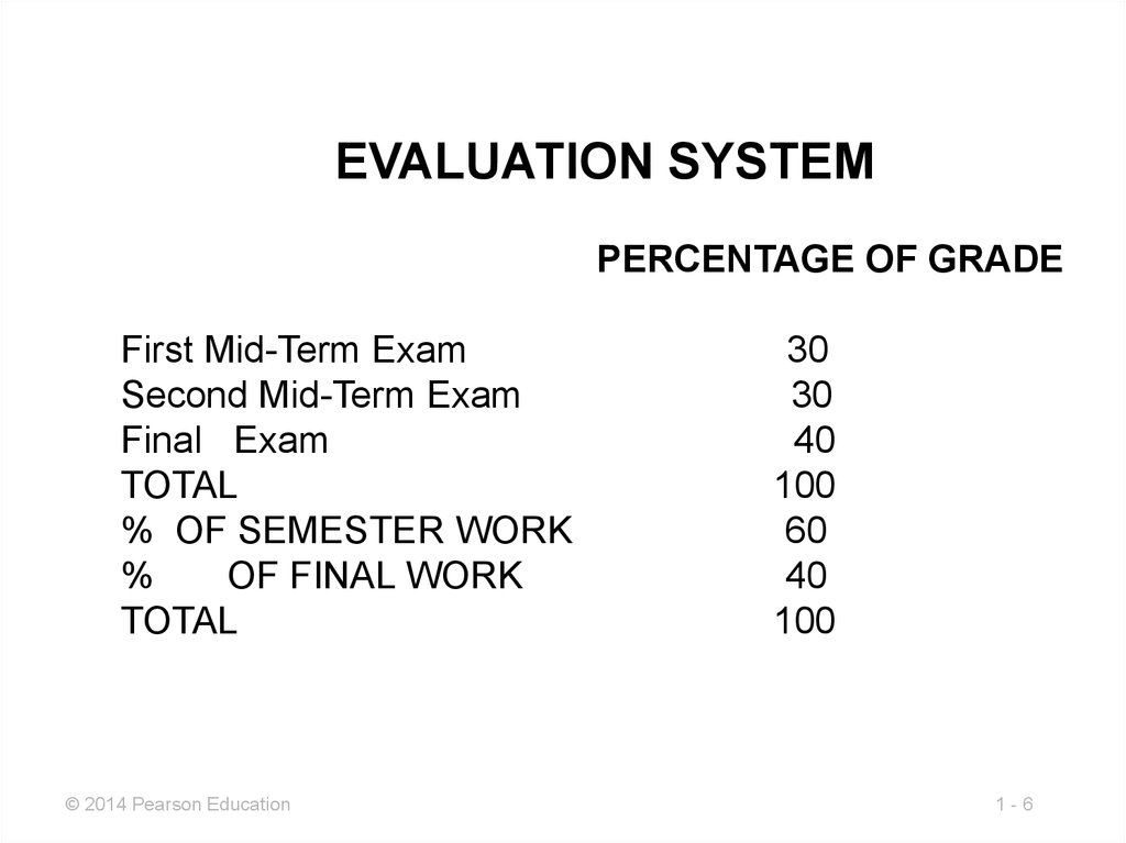
6.

EVALUATION SYSTEM
PERCENTAGE OF GRADE
First Mid-Term Exam
Second Mid-Term Exam
Final Exam
TOTAL
% OF SEMESTER WORK
%
OF FINAL WORK
TOTAL
© 2014 Pearson Education
30
30
40
100
60
40
100
1-6

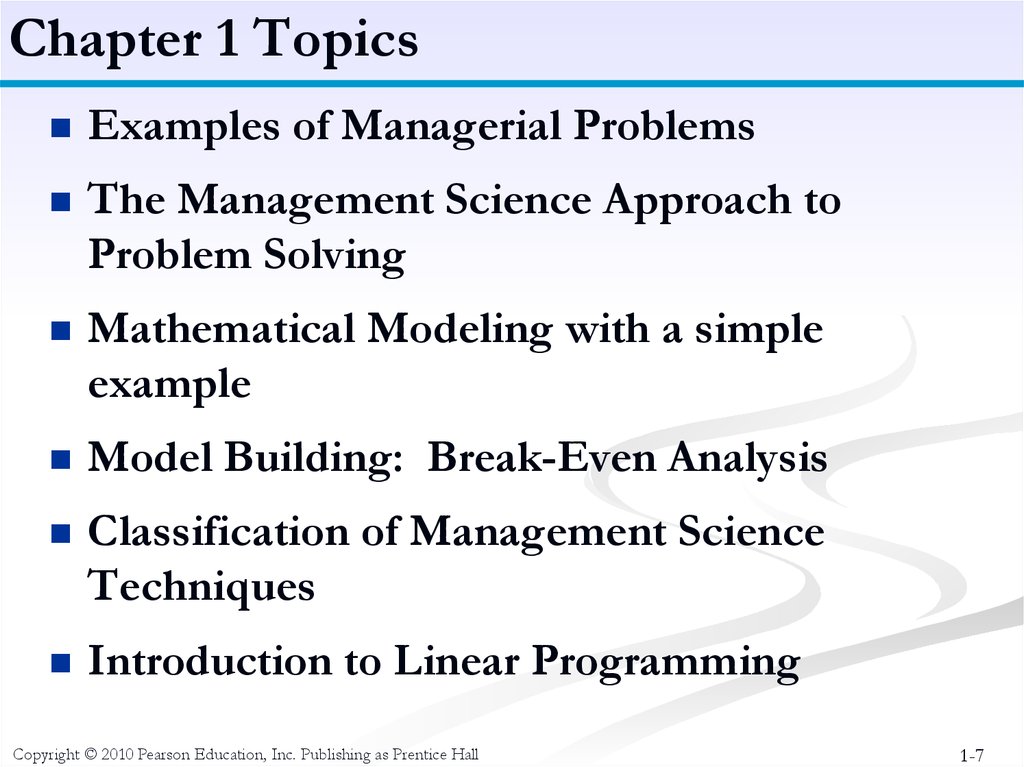
7. Chapter 1 Topics

Examples of Managerial Problems
The Management Science Approach to
Problem Solving
Mathematical Modeling with a simple
example
Model Building: Break-Even Analysis
Classification of Management Science
Techniques
Introduction to Linear Programming
Copyright © 2010 Pearson Education, Inc. Publishing as Prentice Hall
1-7

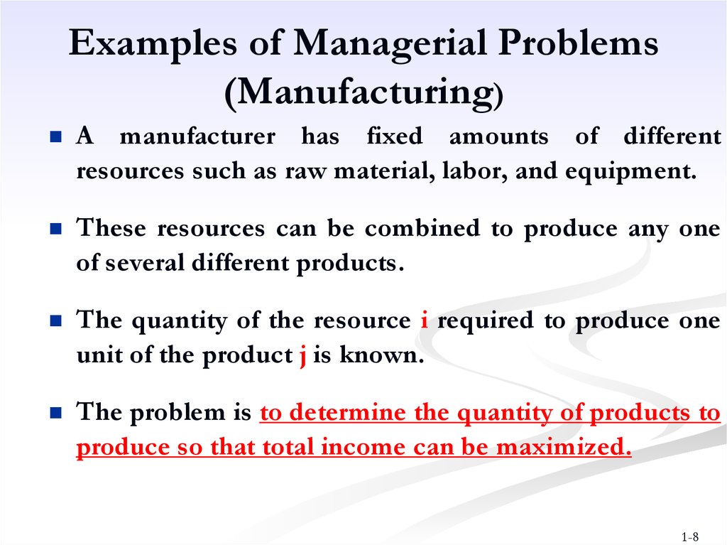
8. Examples of Managerial Problems (Manufacturing)

A manufacturer has fixed amounts of different
resources such as raw material, labor, and equipment.
These resources can be combined to produce any one
of several different products.
The quantity of the resource i required to produce one
unit of the product j is known.
The problem is to determine the quantity of products to
produce so that total income can be maximized.
1-8

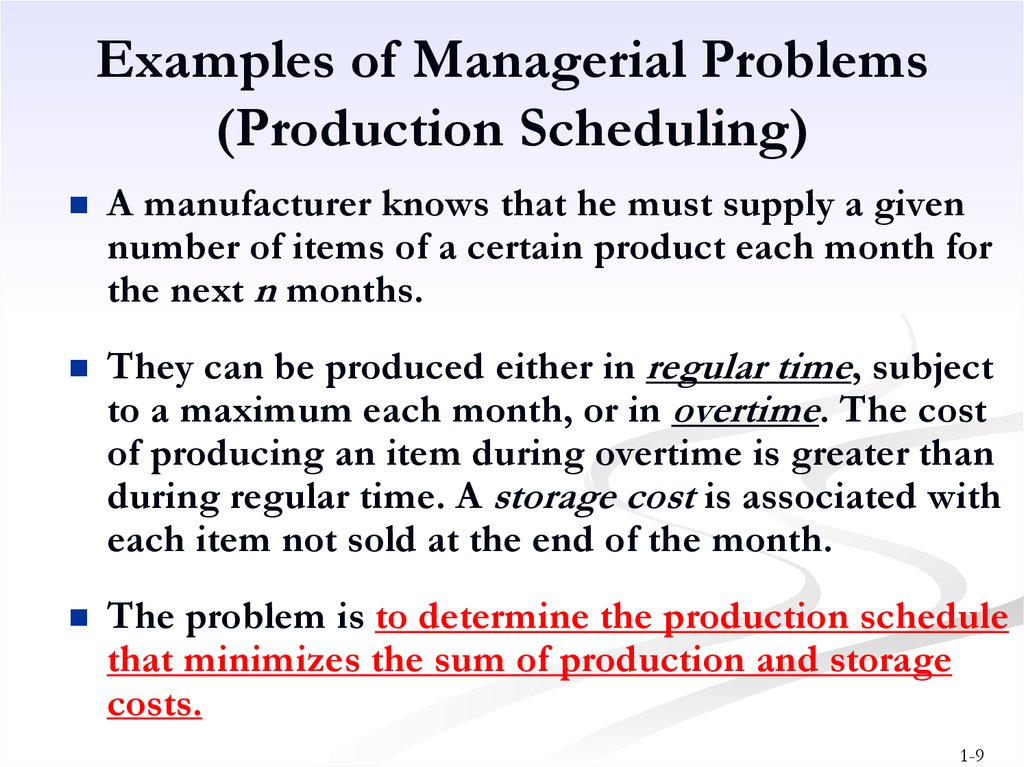
9. Examples of Managerial Problems (Production Scheduling)

A manufacturer knows that he must supply a given
number of items of a certain product each month for
the next n months.
They can be produced either in regular time, subject
to a maximum each month, or in overtime. The cost
of producing an item during overtime is greater than
during regular time. A storage cost is associated with
each item not sold at the end of the month.
The problem is to determine the production schedule
that minimizes the sum of production and storage
costs.
1-9

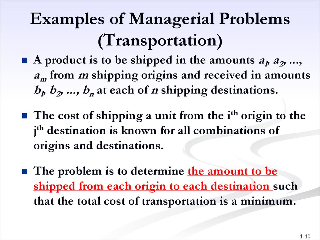
10. Examples of Managerial Problems (Transportation)

A product is to be shipped in the amounts al, a2, ...,
am from m shipping origins and received in amounts
bl, b2, ..., bn at each of n shipping destinations.
The cost of shipping a unit from the ith origin to the
jth destination is known for all combinations of
origins and destinations.
The problem is to determine the amount to be
shipped from each origin to each destination such
that the total cost of transportation is a minimum.
1-10

11.

Examples of Managerial Problems
(Finance: Portfolio Selection Problem)
Alternative investments (shares, bonds, etc.)
Mutual funds, credit unions, banks,
insurance companies
Maximization of expected return
Minimization of risk
___________________________________________________________________________
Operations Research
Jan Fábry 1-11

12.

Examples of Managerial Problems
(Marketing Research)
Evaluating consumer’s reaction to new products
and services
Prepare a campaign with door-to-door personal
interviews about households’ opinion
Households:
with children
without children
Time of interview: daytime, evening
___________________________________________________________________________
Operations Research
Jan Fábry 1-12

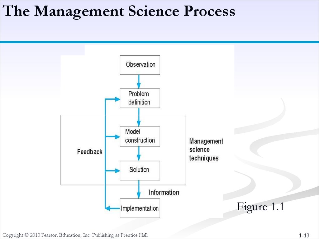
13. The Management Science Process

Figure 1.1
Copyright © 2010 Pearson Education, Inc. Publishing as Prentice Hall
1-13

14.

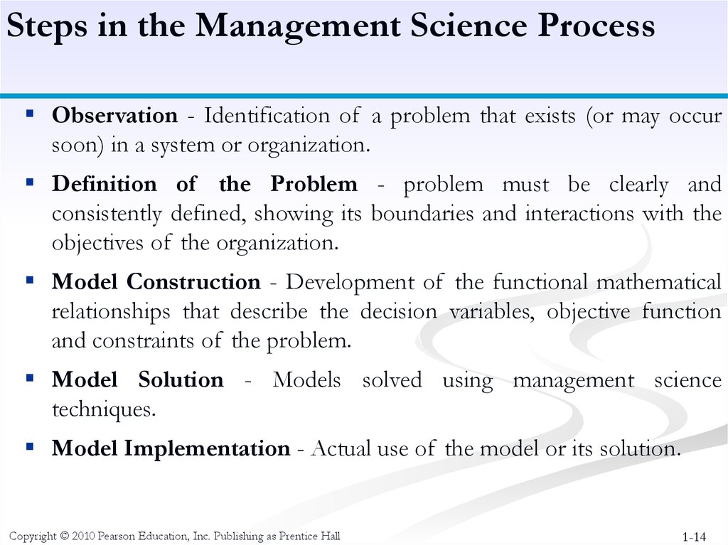
Steps in the Management Science Process
Observation - Identification of a problem that exists (or may occur
soon) in a system or organization.
Definition of the Problem - problem must be clearly and
consistently defined, showing its boundaries and interactions with the
objectives of the organization.
Model Construction - Development of the functional mathematical
relationships that describe the decision variables, objective function
and constraints of the problem.
Model Solution - Models solved using management science
techniques.
Model Implementation - Actual use of the model or its solution.
Copyright © 2010 Pearson Education, Inc. Publishing as Prentice Hall
1-14

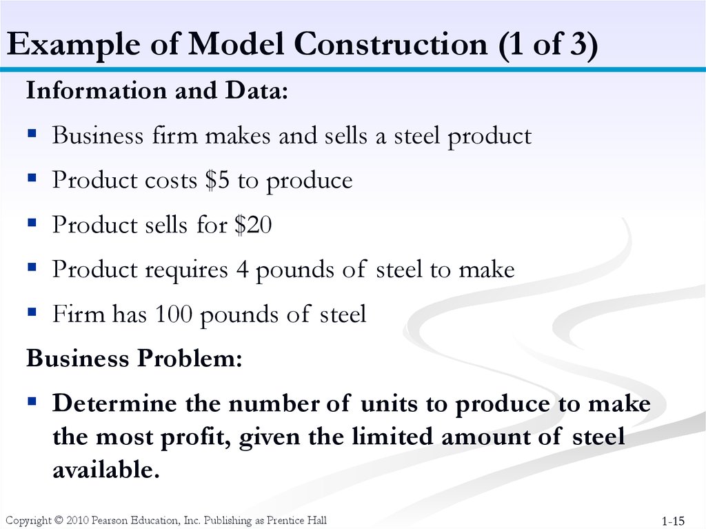
15. Example of Model Construction (1 of 3)

Information and Data:
Business firm makes and sells a steel product
Product costs $5 to produce
Product sells for $20
Product requires 4 pounds of steel to make
Firm has 100 pounds of steel
Business Problem:
Determine the number of units to produce to make
the most profit, given the limited amount of steel
available.
Copyright © 2010 Pearson Education, Inc. Publishing as Prentice Hall
1-15

16.

Example of Model Construction (2 of 3)
Variables:
X = # units to produce (decision variable)
Z = total profit (in $)
Model:
Z = $20X - $5X (objective function)
4X = 100 lb of steel (resource constraint)
Parameters:
$20, $5, 4 lbs, 100 lbs (known values)
Formal Specification of Model:
maximize Z = $20X - $5X
subject to 4X = 100
Copyright © 2010 Pearson Education, Inc. Publishing as Prentice Hall
1-16

17.

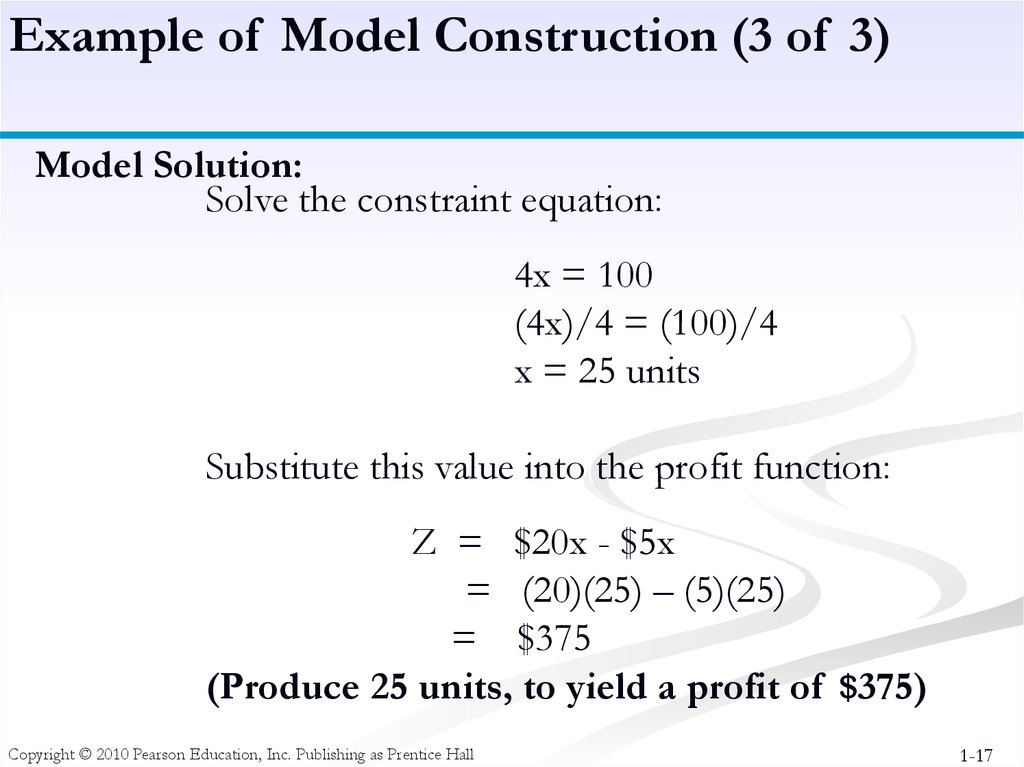
Example of Model Construction (3 of 3)
Model Solution:
Solve the constraint equation:
4x = 100
(4x)/4 = (100)/4
x = 25 units
Substitute this value into the profit function:
Z = $20x - $5x
= (20)(25) – (5)(25)
= $375
(Produce 25 units, to yield a profit of $375)
Copyright © 2010 Pearson Education, Inc. Publishing as Prentice Hall
1-17

18.

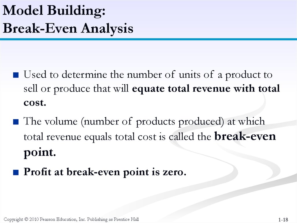
Model Building:
Break-Even Analysis
■ Used to determine the number of units of a product to
sell or produce that will equate total revenue with total
cost.
■ The volume (number of products produced) at which
total revenue equals total cost is called the break-even
point.
■ Profit at break-even point is zero.
Copyright © 2010 Pearson Education, Inc. Publishing as Prentice Hall
1-18

19.

Model Building:
Break-Even Analysis
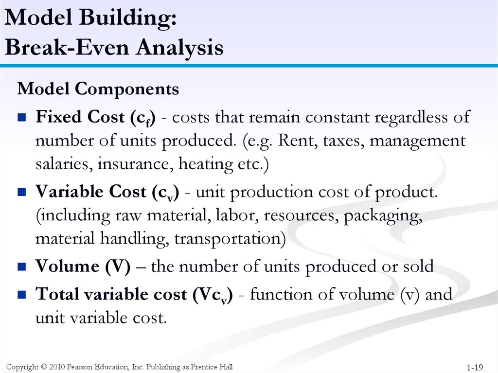
Model Components
Fixed Cost (cf) - costs that remain constant regardless of
number of units produced. (e.g. Rent, taxes, management
salaries, insurance, heating etc.)
Variable Cost (cv) - unit production cost of product.
(including raw material, labor, resources, packaging,
material handling, transportation)
Volume (V) – the number of units produced or sold
Total variable cost (Vcv) - function of volume (v) and
unit variable cost.
Copyright © 2010 Pearson Education, Inc. Publishing as Prentice Hall
1-19

20.

Model Building:
Break-Even Analysis
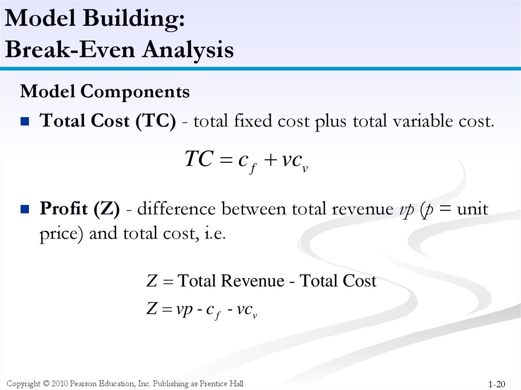
Model Components
Total Cost (TC) - total fixed cost plus total variable cost.
TC c f vcv
Profit (Z) - difference between total revenue vp (p = unit
price) and total cost, i.e.
Z Total Revenue - Total Cost
Z vp - c f - vcv
Copyright © 2010 Pearson Education, Inc. Publishing as Prentice Hall
1-20

21.

Model Building:
Break-Even Analysis
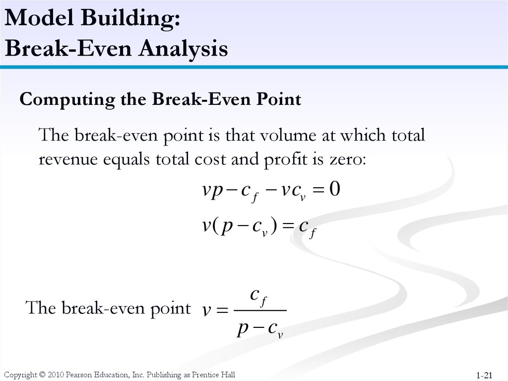
Computing the Break-Even Point
The break-even point is that volume at which total
revenue equals total cost and profit is zero:
vp c f vcv 0
v( p cv ) c f
The break-even point v
Copyright © 2010 Pearson Education, Inc. Publishing as Prentice Hall
cf
p cv
1-21

22.

Model Building:
Break-Even Analysis
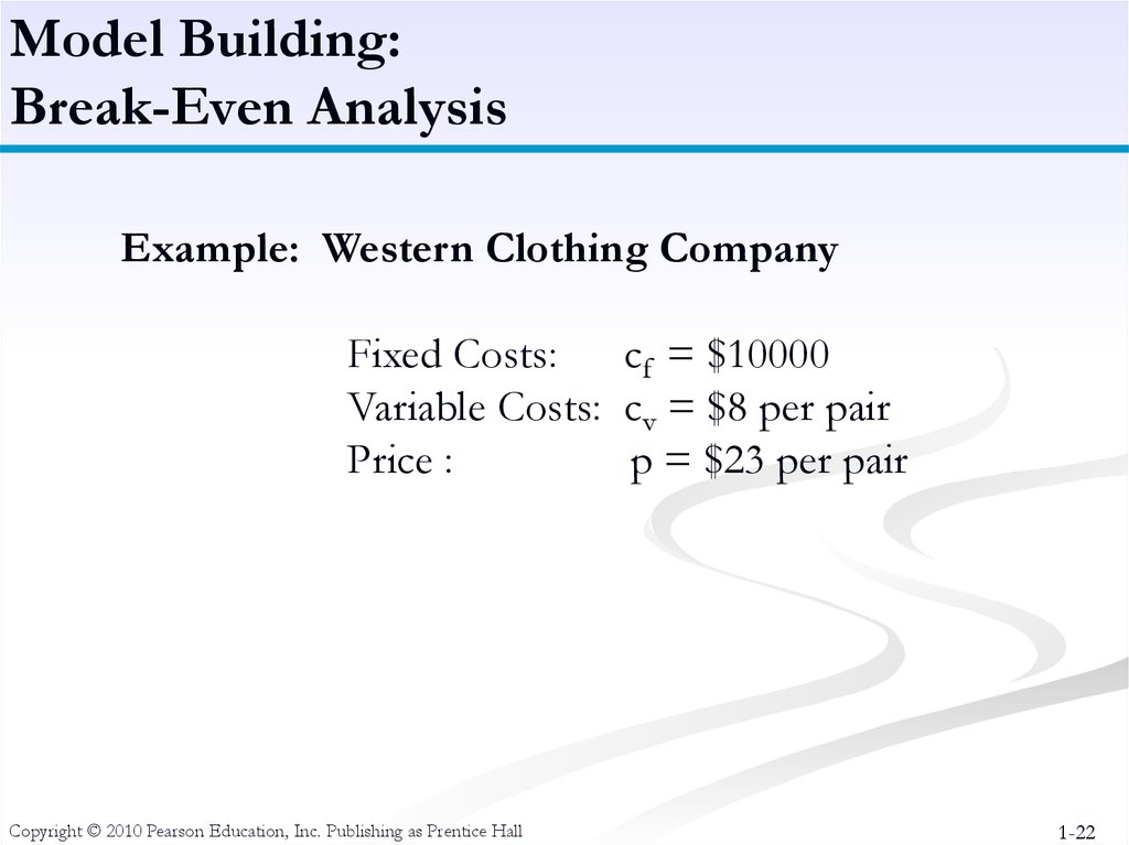
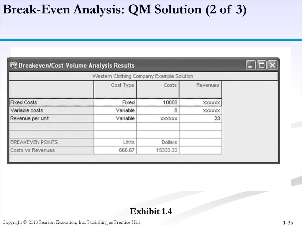
Example: Western Clothing Company
Fixed Costs:
cf = $10000
Variable Costs: cv = $8 per pair
Price :
p = $23 per pair
Copyright © 2010 Pearson Education, Inc. Publishing as Prentice Hall
1-22

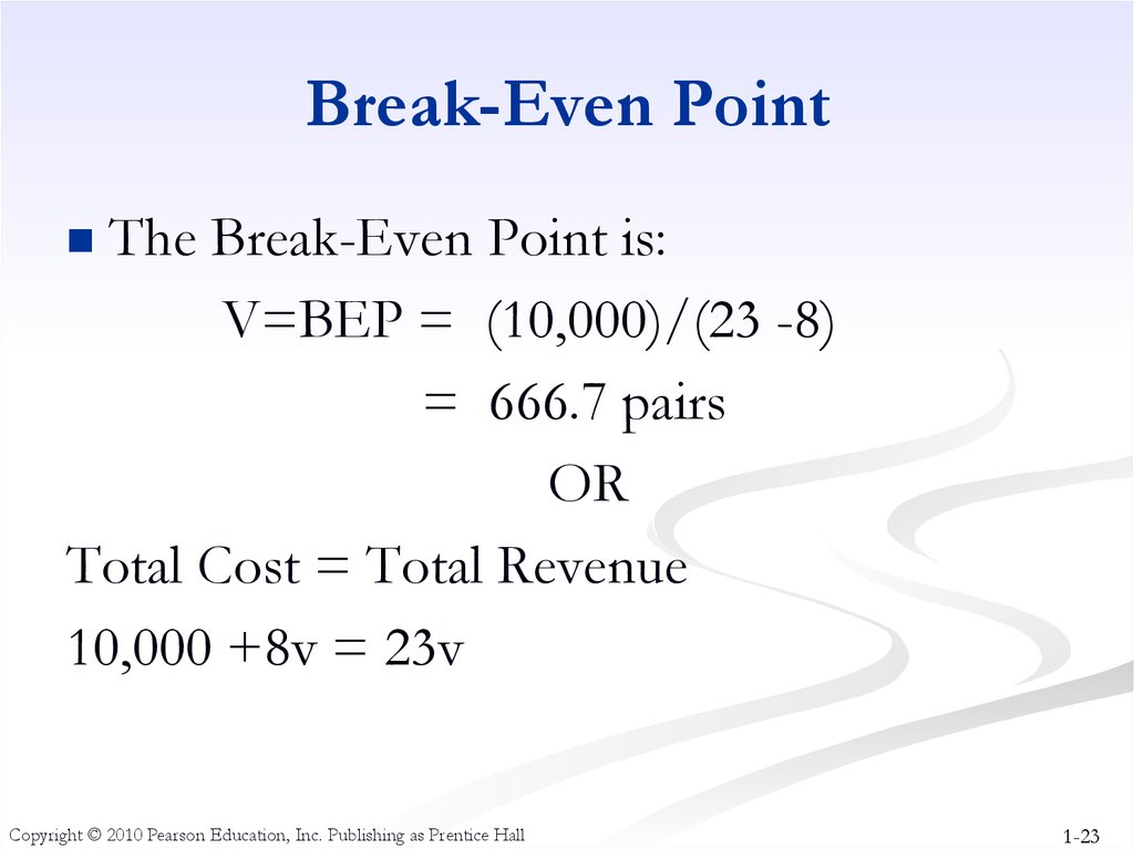
23. Break-Even Point

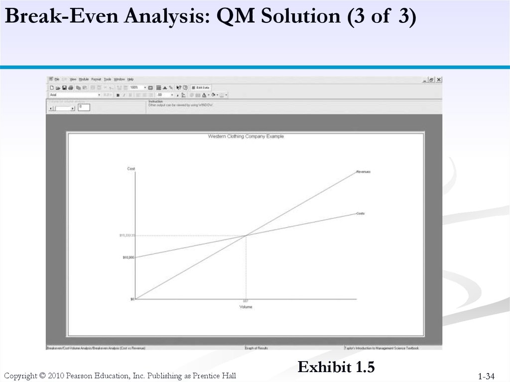
The Break-Even Point is:
V=BEP = (10,000)/(23 -8)
= 666.7 pairs
OR
Total Cost = Total Revenue
10,000 +8v = 23v
Copyright © 2010 Pearson Education, Inc. Publishing as Prentice Hall
1-23

24.

Model Building:
Break-Even Analysis
Figure 1.2
Copyright © 2010 Pearson Education, Inc. Publishing as Prentice Hall
1-24

25.

Model Building:
Break-Even Analysis
Example: Western Clothing Company
Fixed Costs:
cf = $10000
Variable Costs: cv = $8 per pair
Price :
p = $30 per pair
Copyright © 2010 Pearson Education, Inc. Publishing as Prentice Hall
1-25

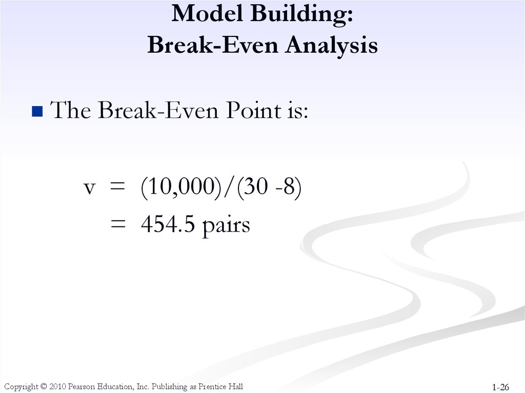
26. Model Building: Break-Even Analysis

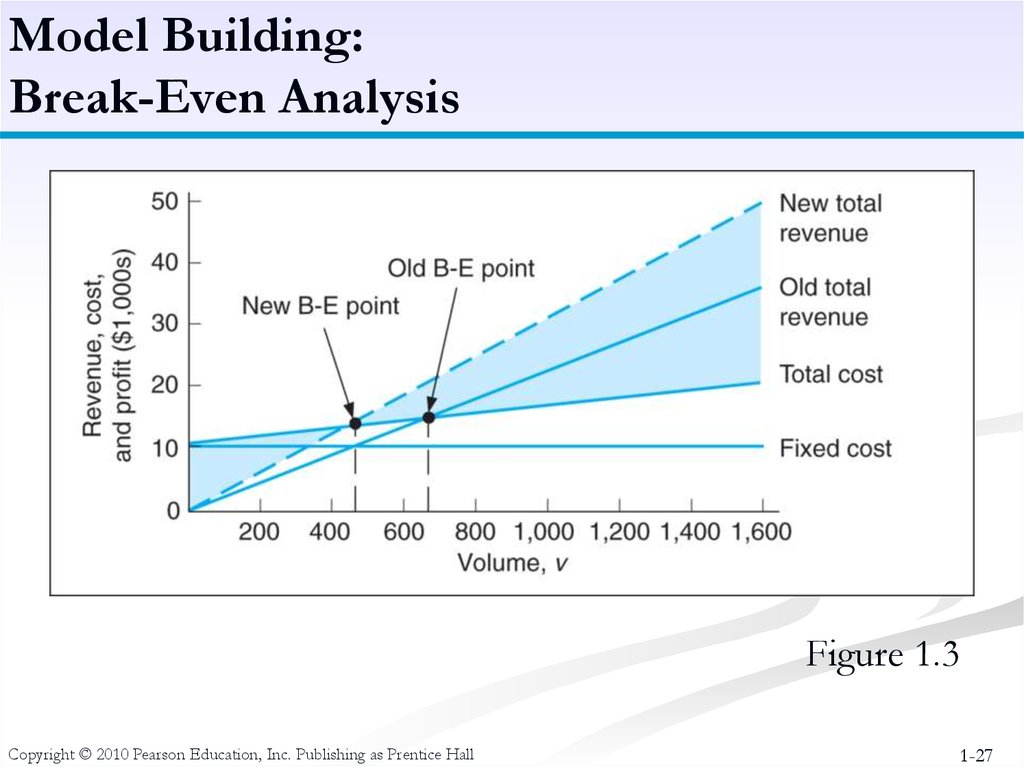
The Break-Even Point is:
v = (10,000)/(30 -8)
= 454.5 pairs
Copyright © 2010 Pearson Education, Inc. Publishing as Prentice Hall
1-26

27.

Model Building:
Break-Even Analysis
Figure 1.3
Copyright © 2010 Pearson Education, Inc. Publishing as Prentice Hall
1-27

28.

Model Building:
Break-Even Analysis
Example: Western Clothing Company
Fixed Costs:
cf = $10000
Variable Costs: cv = $12 per pair
Price :
p = $30 per pair
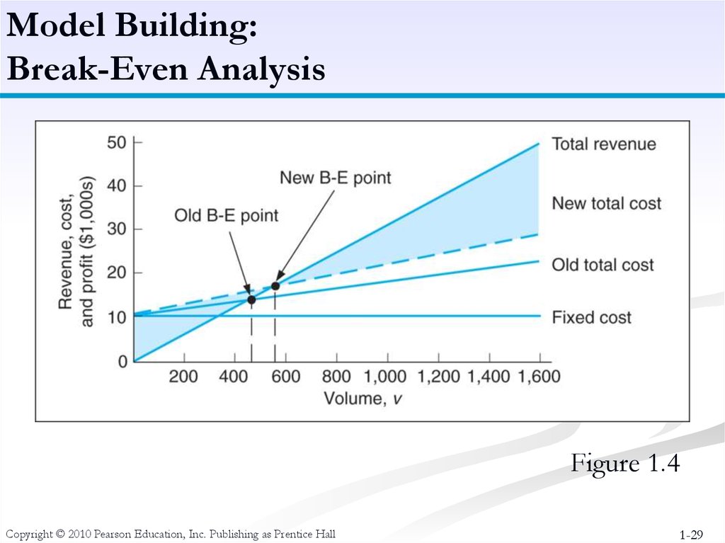
The Break-Even Point is:
v = (10,000)/(30 -12)
= 555.5 pairs
Copyright © 2010 Pearson Education, Inc. Publishing as Prentice Hall
1-28

29.

Model Building:
Break-Even Analysis
Figure 1.4
Copyright © 2010 Pearson Education, Inc. Publishing as Prentice Hall
1-29

30.

Model Building:
Break-Even Analysis
Example: Western Clothing Company
Fixed Costs:
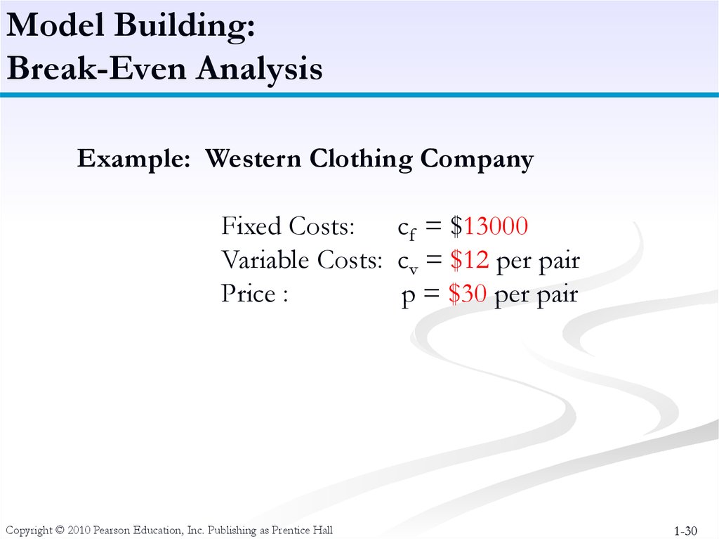
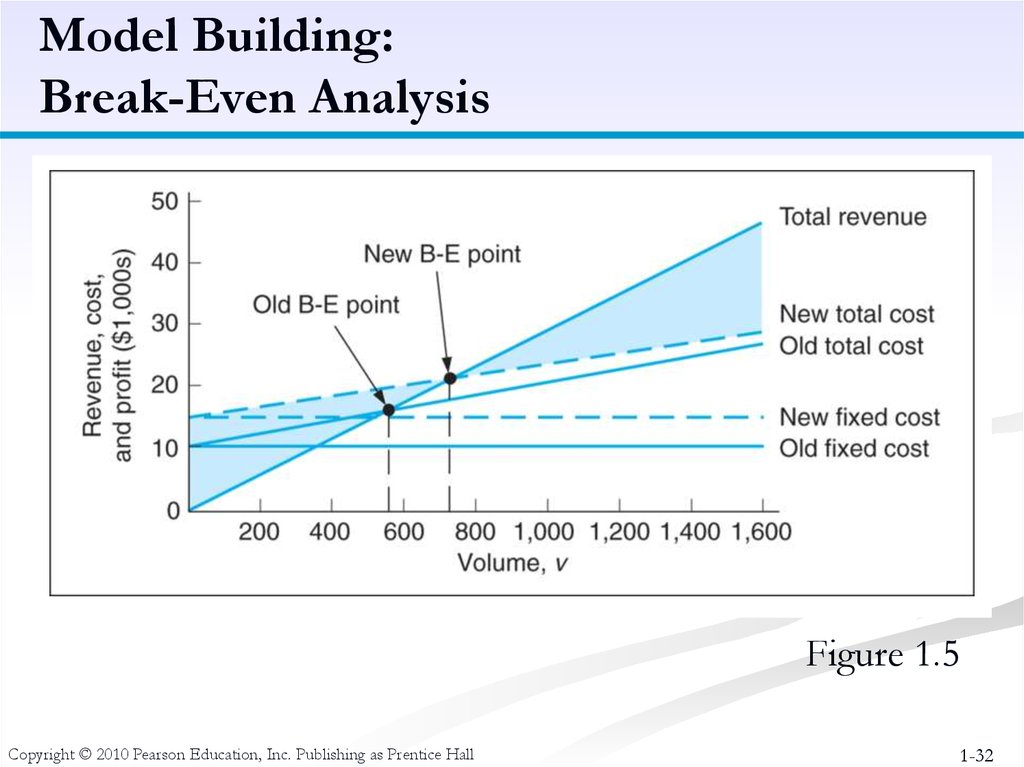
cf = $13000
Variable Costs: cv = $12 per pair
Price :
p = $30 per pair
Copyright © 2010 Pearson Education, Inc. Publishing as Prentice Hall
1-30

31. Model Building: Break-Even Analysis

The Break-Even Point is:
v = (13,000)/(30 -12)
= 722.2 pairs
Copyright © 2010 Pearson Education, Inc. Publishing as Prentice Hall
1-31

32.

Model Building:
Break-Even Analysis
Figure 1.5
Copyright © 2010 Pearson Education, Inc. Publishing as Prentice Hall
1-32

33.

Break-Even Analysis: QM Solution (2 of 3)
Exhibit 1.4
Copyright © 2010 Pearson Education, Inc. Publishing as Prentice Hall
1-33

34.

Break-Even Analysis: QM Solution (3 of 3)
Copyright © 2010 Pearson Education, Inc. Publishing as Prentice Hall
Exhibit 1.5
1-34

35.

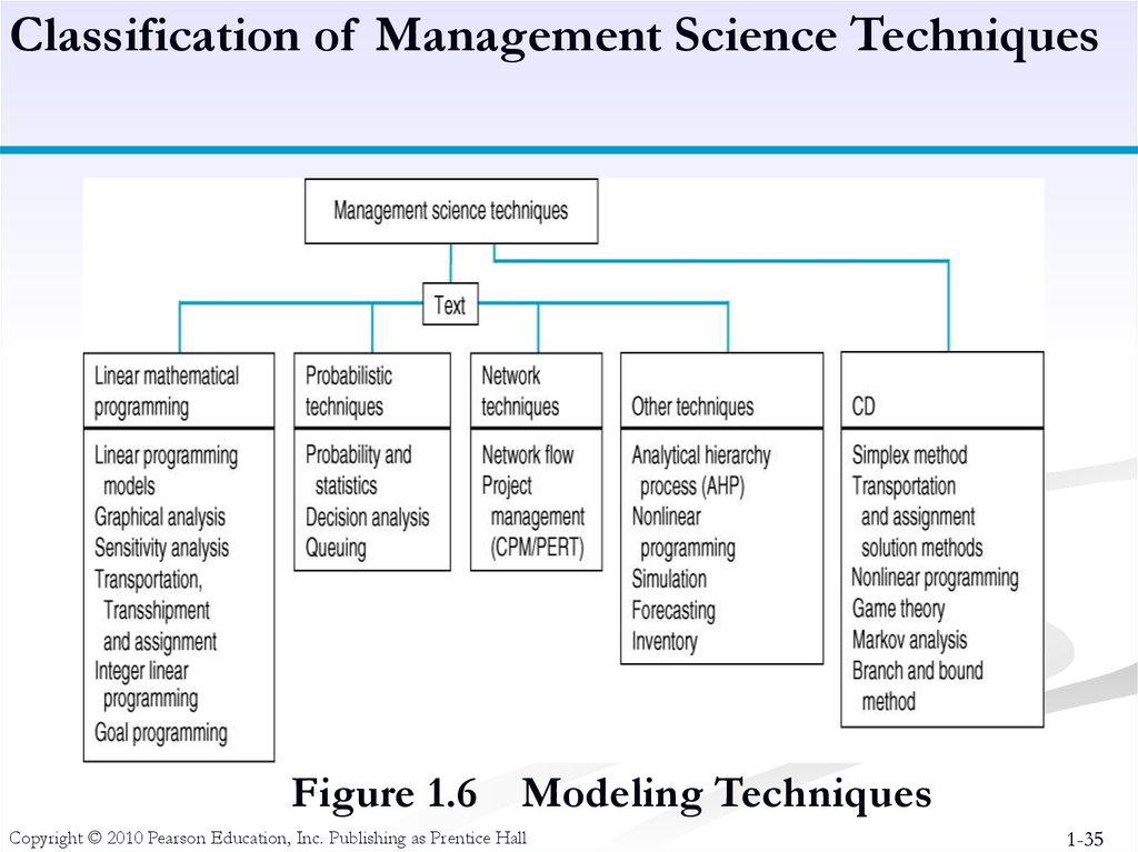
Classification of Management Science Techniques
Figure 1.6
Modeling Techniques
Copyright © 2010 Pearson Education, Inc. Publishing as Prentice Hall
1-35

36.

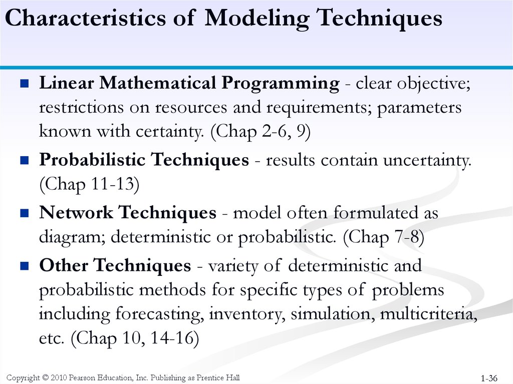
Characteristics of Modeling Techniques
Linear Mathematical Programming - clear objective;
restrictions on resources and requirements; parameters
known with certainty. (Chap 2-6, 9)
Probabilistic Techniques - results contain uncertainty.
(Chap 11-13)
Network Techniques - model often formulated as
diagram; deterministic or probabilistic. (Chap 7-8)
Other Techniques - variety of deterministic and
probabilistic methods for specific types of problems
including forecasting, inventory, simulation, multicriteria,
etc. (Chap 10, 14-16)
Copyright © 2010 Pearson Education, Inc. Publishing as Prentice Hall
1-36

37. The Linear Programming Model (1)

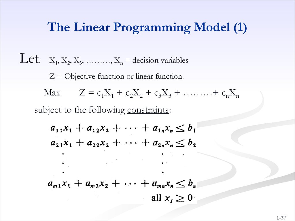
Let:
X1, X2, X3, ………, Xn = decision variables
Z = Objective function or linear function.
Max
Z = c1X1 + c2X2 + c3X3 + ………+ cnXn
subject to the following constraints:
where aij, bi, and cj are given constants.
1-37

38. The Linear Programming Model (2)

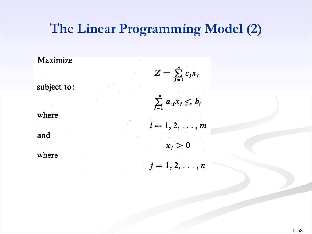
…..Eq (3)
1-38