Aggregated supply and demand

1. Macroeconomics aggregated supply and demand

MACROECONOMICS
AGGREGATED SUPPLY AND
DEMAND
Zharova Liubov

2. Aggregate Demand (AD)

AGGREGATE DEMAND (AD)
Aggregate demand is the total demand for goods and services
is an economic measurement of the sum of all final goods and
services produced in an economy, expressed as the total amount of
money exchanged for those goods and services.
macro
micro
Demand
P
Q
P
AD = total spending on goods
and services = Real GDP
Aggregate AD = C+I+G+NX
Demand
Real GDP
1. Wealth effect
2. Savings and Interest rate effect
3. Foreign exchange effect
C - Consumer spending on goods
and services
I - Private investment and
corporate spending for nonfinal capital goods (factories,
equipment, etc.)
G - Government spending for
public goods and social services
(infrastructure, Medicare, etc.)
NX = Net
exports (exports minus imports)

3. AD shifts

AD SHIFTS
AD = C+I+G+NX
change in consumption
(eg cut tax)
Or tax increasing
P
Shifts in
Real GDP
Investment
Governmental spending
Export

4. Components of AS

AGGREGATE SUPPLY (AS)
(or total output) is the total supply of goods and services
produced within an economy at a given overall price
level in a given time period.
COMPONENTS OF AS
Consumer goods. Private consumer goods and services, such as motor
vehicles, computers, clothes and entertainment, are supplied by
the private sector, and consumed by households.
Capital goods. Capital goods, such as machinery, equipment, and
plant, are supplied to other firms.
Public and merit goods. Goods and services produced by private
firms for use by central or local government, such
as education and healthcare, are also a significant component of
aggregate supply.
Traded goods. Goods and services for export, such as chemicals,
entertainment, and financial services are also a key component of
aggregate supply.

5.

LONG-RUN AGGREGATE SUPPLY (LRAS)
Supply = capability to produce
Population growth
Easy to find a job (training…)
More productive (new resources…)
…
War, conflicts …
P
Real GDP
Maximum
productivity
P
Natural level of
productivity
Real GDP

6. Sort-run Aggregate Supply (SRAS)

SORT-RUN AGGREGATE SUPPLY (SRAS)
SRAS
Rising the price – labor pool,
work more, less vacation…
Decreasing price – more leisure
time…
Curren
t prices
P
LRAS
Real GDP
Shape
1. Misperception theory:
2. Sticky wages (cost/prices) theory

7. Summirising

SUMMIRISING
Aggregate supply is the total quantity of output firms will
produce and sell – in other words, the real GDP.
The upward-sloping aggregate supply curve – also known
as the short run aggregate supply curve – shows the
positive relationship between price level and real GDP in the
short run.
The aggregate supply curve slopes up because when the price
level for outputs increases while the price level of inputs
remains fixed, the opportunity for additional profits
encourages more production.
Potential GDP, or full-employment GDP, is the maximum
quantity that an economy can produce given full employment
of its existing levels of labor, physical capital, technology, and
institutions.
Aggregate demand is the amount of total spending on
domestic goods and services in an economy.
The downward-sloping aggregate demand curve shows the
relationship between the price level for outputs and the
quantity of total spending in the economy.

8. Equilibrium in the aggregate demand/aggregate supply model

EQUILIBRIUM IN THE AGGREGATE
DEMAND/AGGREGATE SUPPLY MODEL
LRAS
AD
SRAS
P
E
Real GDP
At a relatively low price level for
output, firms have little incentive to
produce, although consumers would
be willing to purchase a high
quantity. As the price level for
outputs rises, aggregate supply rises
and aggregate demand falls until the
equilibrium point is reached.
Conclusions
If equilibrium occurs in the flat range of AS, then economy is
not close to potential GDP and will be experiencing
unemployment but stable price level. If equilibrium occurs in
the steep range of AS, then the economy is close to or at
potential GDP and will be experiencing rising price levels or
inflationary pressures, but will have a low unemployment
rate.

9. Price level: aggregate demand/aggregate supply

PRICE LEVEL: AGGREGATE
DEMAND/AGGREGATE SUPPLY
Conclusions: the equilibrium is fairly far from where the AS
curve becomes steep. This implies that the economy is not close
to potential GDP. Thus, unemployment will be high, and
changes in the price level are likely to be small.

10. Example

EXAMPLE
Bebebe. The imaginary country of Bebebe has
the aggregate supply and aggregate demand
curves given in the table below.
Plot an AD/AS diagram from the data above.
Identify the equilibrium.
Would you expect unemployment in this
economy to be relatively high or low? Would
you expect concern about inflation in this
economy to be relatively high or low?
Imagine that consumers begin to lose
confidence about the state of the economy, so
AD becomes lower by 275 at every price level.
Identify the new aggregate equilibrium. How
will the shift in AD affect the original output,
price level, and employment?

11. How productivity growth shifts the AS curve

HOW PRODUCTIVITY GROWTH SHIFTS THE
AS CURVE
Over time, productivity grows so that the same
quantity of labor can produce more output.
Historically, the real growth in GDP per capita in
an advanced economy like the United States has
averaged about 2% to 3% per year, but
productivity growth has been faster during
certain extended periods.
A higher level of productivity shifts the SRAS
curve to the right because with improved
productivity, firms can produce a greater
quantity of output at every price level.

12.

13. Summary

SUMMARY
The aggregate demand/aggregate supply model is a model
that shows what determines total supply or total demand
for the economy and how total demand and total supply
interact at the macroeconomic level.
Movements of either the aggregate supply or aggregate
demand curve in an AD/AS diagram will result in a
different equilibrium output and price level.
The aggregate supply curve shifts to the right as
productivity increases or the price of key inputs falls,
making a combination of lower inflation, higher output,
and lower unemployment possible.
The aggregate supply curve shifts to the left as the price of
key inputs rises, making a combination of lower output,
higher unemployment, and higher inflation possible.
When an economy experiences stagnant growth and high
inflation at the same time it is referred to as stagflation.

14. How do changes by consumers and firms affect AD?

HOW DO CHANGES BY CONSUMERS AND
FIRMS AFFECT AD?
When consumers feel more confident about the future
of the economy, they tend to consume more. If
business confidence is high, then firms tend to spend
more on investment, believing that the future payoff
from that investment will be substantial. On the
other hand, if consumer or business confidence drops,
then consumption and investment spending decline.
Consumer and business confidence often reflect
macroeconomic realities. For example, confidence is
usually high when the economy is growing briskly
and low during a recession. However, economic
confidence can sometimes rise or fall due to factors
that do not have a close connection to the immediate
economy, like a risk of war, election results, foreign
policy events, or a pessimistic prediction about the
future by a prominent public figure.

15.

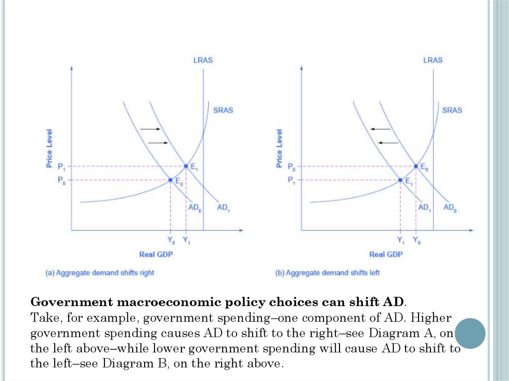
Government macroeconomic policy choices can shift AD.
Take, for example, government spending–one component of AD. Higher
government spending causes AD to shift to the right–see Diagram A, on
the left above–while lower government spending will cause AD to shift to
the left–see Diagram B, on the right above.

16.

During a recession, when
unemployment is high and many
businesses are suffering low
profits or even losses, the US
Congress often passes tax cuts.
During the recession of 2001, for
example, a tax cut was enacted
into law. At such times, the
political rhetoric often focuses on
how people going through hard
times need relief from taxes. The
aggregate supply and aggregate
demand framework, however,
offers a complementary rationale.
The original equilibrium during the recession is at point E0 relatively
far from the full-employment level of output. The tax cut, by increasing
consumption, shifts the AD curve to the right. At the new equilibrium
E1 real GDP rises and unemployment falls and – because in this
diagram the economy has not yet reached its potential or fullemployment level of GDP – any rise in the price level remains muted.

17. Summary

SUMMARY
The aggregate demand/aggregate supply model is a model that
shows what determines total supply or total demand for the
economy and how total demand and total supply interact at the
macroeconomic level.
The aggregate demand curve shifts to the right as the components
of aggregate demand–consumption spending, investment
spending, government spending, and spending on exports minus
imports–rise. The AD curve will shift back to the left as these
components fall.
AD components can change because of different personal choices–
like those resulting from consumer or business confidence–or from
policy choices like changes in government spending and taxes.
If the AD curve shifts to the right, then the equilibrium quantity
of output and the price level will rise. If the AD curve shifts to the
left, then the equilibrium quantity of output and the price level
will fall.
Whether equilibrium output changes relatively more than the
price level or whether the price level changes relatively more than
output is determined by where the AD curve intersects with the
AS curve.