Demand 11.2a

1. Demand 11.2a

03/09/2018
Sonali Sinha Roy
1

2. Learning Objectives

By the end of the lesson the learners will be able to :
Define and understand the terms
Demand
Movement along and shift in the demand curves
Substitute goods
Complementary goods.
Analyse and apply the concept to real world situation .
(1 min)

3. Demand

Willingness to Buy
Ability to Pay

4. Demand Schedule

PRICE ($)
Quantity Demanded
for Eggs
10
9
5
14
8
7
6
16
22
26
5
4
32
42
3
49
2
1
62
80
03/09/2018
Sonali Sinha Roy
4

5. Downward slope of Demand Curve

Law of Demand:
The negative
relationship
between the price
of a good and the
quantity demanded,
when all other
factors that
influence demand
are held fixed.
03/09/2018
Sonali Sinha Roy
5

6. Reason for Downward Sloping Demand Curve

Income and substitution effects
The negative slope of the demand curve is due to the substitution and
income effects.
If the relative price of a good falls consumers will substitute that good
for more expensive goods -that will buy more of the good whose
relative price has fallen and less of the other goods. This is the
substitution effect.
When the relative price of a good falls the consumer can buy the same
bundle of goods as before the price decline and have some money left
over. This money can be used to purchase more of all his consumption
goods. In other words his purchasing power is called the income effect
03/09/2018
Sonali Sinha Roy
6

7. Movement along the Demand Curve

Movement along the Demand curve
is due to the change in price only.
Other factors are kept constant .
Movement from Point A to B:
Extension in Demand/Increase in
Quantity Demanded - P ↓ QD ↑
Movement from Point C to B:
Contraction in Demand/Decrease in
Quantity Demanded - P ↑QD ↓
03/09/2018
Sonali Sinha Roy
7

8. Shift in Demand

PINTE:
P = Price of the related goods
I = Income of the consumer
N = Number of buyers
T = Taste & Preference
E = Expectation of price in future
03/09/2018
Sonali Sinha Roy
8

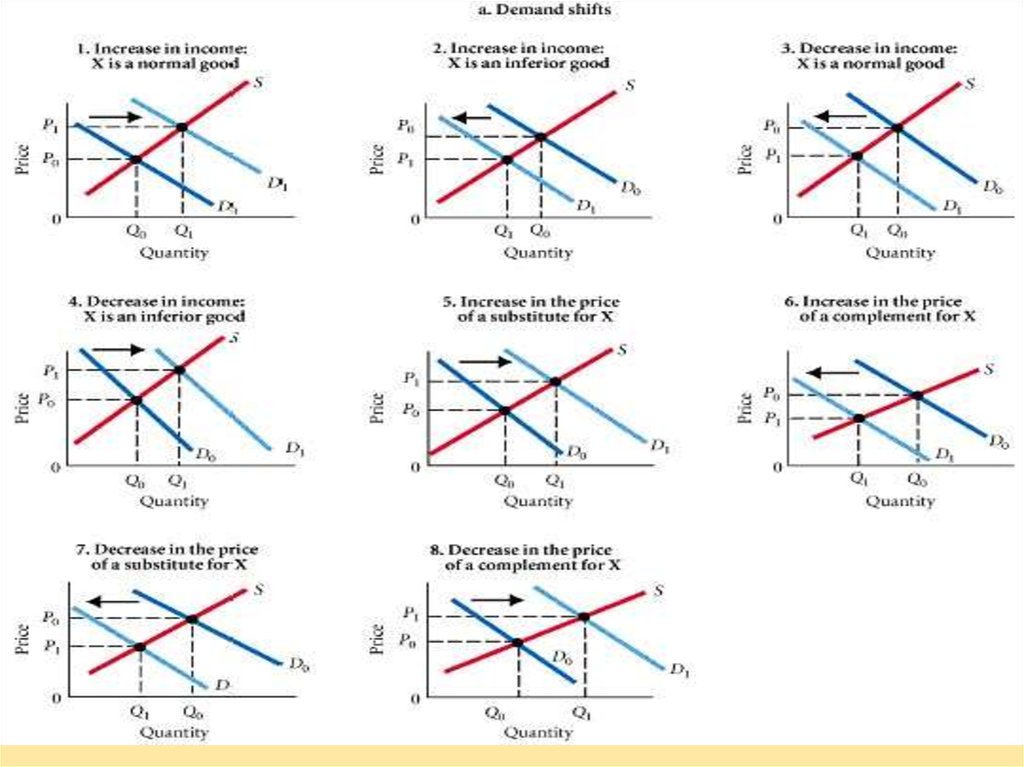
9. Identify from the following: Normal & Inferior Goods ; Complementary & Substitute Goods

Identify from the following: Normal & Inferior Goods ;
Complementary & Substitute Goods
03/09/2018
Sonali Sinha Roy
9

10. Shifts in Demand Curve

03/09/2018
Sonali Sinha Roy
10

11.

03/09/2018
Sonali Sinha Roy
11

12. Recap of Today’s Lesson

03/09/2018
Sonali Sinha Roy
12

13. Reflection

03/09/2018
Sonali Sinha Roy
13

14. Demand 11.2a

03/09/2018
Sonali Sinha Roy
14

15. Learning Objectives

By the end of the lesson the learners will be able to :
Define and understand the terms
Demand Function
Plot demand curve with the help of a given equation
Analyse and apply the concept to real world situation .
(1 min)

16. Demand Function

Indirect relationship between Price and Quantity
Demanded
QD P
Equation:
Qd = a – bP
Qd = quantity of a good demanded
P is the price of the good
a = vertical intercept (Max QD )
b = the slope of the demand curve
P = (a/b) – (Q/b)
03/09/2018
Sonali Sinha Roy
16

17. Example

Price
Demand: Q = 100 -2P
Inverse Demand: P = 50 – (Q/2)
• The vertical intercept is
therefore 50 and represents the
Price
a/b
50
P = (a/b) - (Q/b)
P = 50- (Q/2)
• The horizontal intercept is
therefore 100 , and represents
the amount of the good the
consumer would want to
purchase at a price of 0.
100
0
Quantity Demanded
Demand: Q = a – bP
Inverse Demand: P = (a/b) – (Q/b)
03/09/2018
Sonali Sinha Roy
17

18. In-class activity

Use the linear demand function for cappuccinos, Qd = 500 – 25P to
answer the questions that follow:
•Create a demand schedule for cappuccinos with the prices of $0, $1,
$3, $5, $7 and $9
•Create a demand curve for cappuccinos, plotting the points from your
demand schedule.
•Assume the price of latte machiatos, a close substitute for cappuccinos,
decreases, and causes the a variable in the demand function to fall to
300. Create a new demand schedule, with the adjusted values for Qd.
•On your previous diagram, illustrate the new demand curve.
•Assume that due to falling incomes, cappuccino consumers become
more sensitive to changes in the price of cappuccinos, and the b variable
in the original demand function increases to 40. Using the same prices,
create a new demand schedule.
•On the same graph as your original demand curve, illustrate the new
demand
for cappuccinos following
decline in consumers’ incomes.
03/09/2018
Sonalithe
Sinha Roy
18

19. Recap of Today’s Lesson

03/09/2018
Sonali Sinha Roy
19

20. Reflection

03/09/2018
Sonali Sinha Roy
20