Deep learning and rses

1.

Recommendation Systems and Deep Learning
Inna Skarga-Bandurova
Computer Science and Engineering Depatrment
V. Dahl East Ukrainian National University
Kharkiv, 17-19 April 2018

2. Structure of Lectures

• Yesterday: Introduction to Deep Learning
• Today: Recommendation Systems and Deep Learning
• Overview of Recommender Systems (RSes)
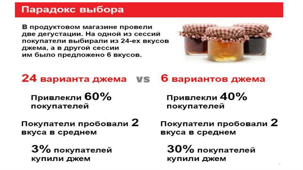
• Paradox of Choice
• The three generations (1G – 3G)
• Overview of some of the application domains
• Tomorrow: Deep Learning for Human-Computer Interaction
This is a lecture series about the challenges (and new opportunities) for ML/DL

3.

3

4. Less is More

4

5. Recommendation Systems: Academia

• Huge progress over the last 20 years
• from the 3 initial papers published in 1995
• to 1000’s of papers now
• Annual ACM RecSys Conference (since 2007)
• E.g., Boston/MIT in 2016, Milan in 2017
• Hundreds of submissions and participants
• Interdisciplinary field, comprising
• CS, data science, statistics, marketing, OR, psychology
• A LOT of interest from industry in the academic research. Usually, 40% of
RecSys participants are from the industry!
• An excellent example of the symbiosis of the academic research and industrial
developments.

6. Recommender Systems in the Industry

• Industry pioneers:
• Amazon, B&N, Net Perceptions (around 1996-1997)
• Hello, Jim, we have recommendations for you!
• Early days of RSes:
• User/item-based collaborative filtering [Linden et al 2003]
• Forrester Research study (2004):
• 7.4% consumers often bought recommended products
• 22% ascribe value to those recommendations
• 42% were not interested in recommended products

7. Today’s Recommenders

• Work across many firms (Netflix, Yelp, Pandora, Google, Facebook, Twitter,
LinkedIn) and they operate differently across various applications supported by
these firms
• Became mission critical [Colson 2014]: they drive
35% of Amazon’s sales
50% of LinkedIn connections
80% of Netflix streamed hours; savings of $1B/yr [GH15]
100% of Stitch Fix sales of its merchandize
• “By 2020, 100% of what is sold in retail will be by recommendation” (Katrina Lake, CEO of Stitch Fix)
• Deploy sophisticated ML, Big Data, DL and other methods that operate at scale
• Conclusion: big progress over the last 15 years!

8. Buy Now or Tomorrow?

Startup
bought by
Microsoft Co.
2011
$210millions
100 employers

9. Three Generations of Recommender Systems

• Overview of the traditional paradigm of RSes (1st generation)
• Current generation of RSes (2nd generation)
• The opportunities and challenges
• Towards the next (3rd) generation of RSes
Based on A. Tuzhilin, NY University

10.

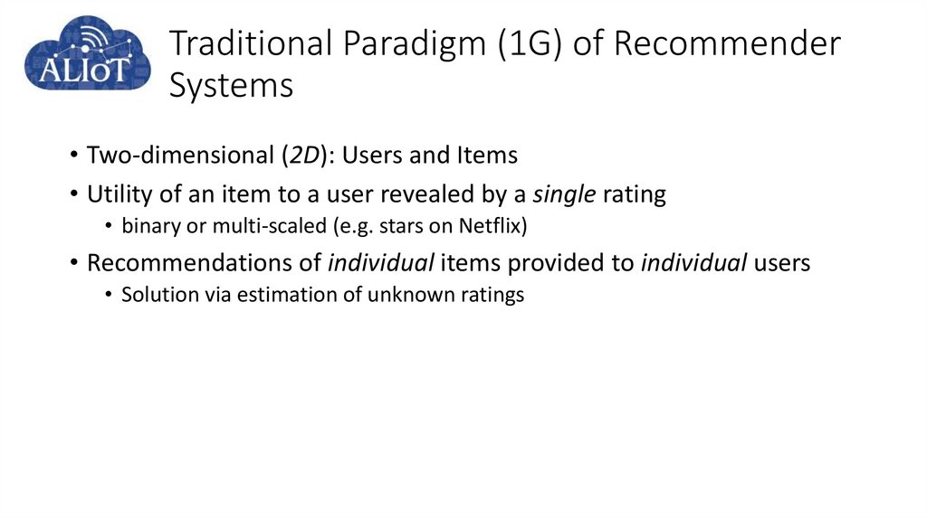
Traditional Paradigm (1G) of Recommender
Systems
• Two-dimensional (2D): Users and Items
• Utility of an item to a user revealed by a single rating
• binary or multi-scaled (e.g. stars on Netflix)
• Recommendations of individual items provided to individual users
• Solution via estimation of unknown ratings

11. 2D Recommendation Matrix

King
Arthur
Water
Life
Brillia
Mind
Avatar
U1
4
3
2
4
U2
?
4
5
5
U3
2
2
4
?
U4
3
?
5
2
• The 2D Users × Items = Matrix of Ratings
• matrix is sparse: only few ratings are specified
• Key issue: accurate estimation of unknown ratings

12. Traditional Approaches

• Input
• Rating matrix R: rij – rating user ci assigns to item sj
• User attribute matrix X: xij – attribute xj of user ci
• Item attribute matrix Y: yij – attribute yj of item si
• Output
• Predicted rating matrix
(predicted utility) R̂
s1
c1
c2
…
cM
…
sN
ˆ f ( R, X , Y )
R
R
x1
c1
c2
…
cM
x2
…
y2
…
Y
s1
xP
c1
c2
…
cM
X
y1
s1
s2
…
sN
s2
yQ
s2
…
R̂
sN

13. Types of Recommendations [Balabanovic & Shoham 1997]

Types of Recommendations [Balabanovic & Shoham 1997]
• Content-based
• build a model based on a description of the item and a
c
profile of the user’s preference, keywords are used to 1
c2
describe the items; beside, a user profile is built to
…
indicate the type of item this user likes.
• Collaborative filtering
• All observed ratings are taken as input to predict
unobserved ratings. Recommend items based only on
the users past behavior
• User-based: Find similar users to me and recommend
what they liked
• Item-based: Find similar items to those that I have
previously liked
• Hybrid
• All observed ratings, item attributes, and user
attributes are taken as input to predict observed
ratings
s1
s2
…
sN
R
cM
x1
c1
c2
…
cM
…
y2
…
Y
s1
xP
c1
c2
…
cM
X
y1
s1
s2
…
sN
x2
yQ
s2
…
R̂
sN

14. Taxonomy of Traditional Recommendation Methods

• Classification based on
• Recommendation approach
• Content-based, collaborative filtering, hybrid
• Nature of the prediction technique
• Heuristic-based, model-based
Heuristic-based
Content-based
Collaborative filtering
Hybrid
Model-based

15. Knowledge Discovery in Databases (KDD) process

Knowledge
Data
Interpretation
and Evaluation
Selection
Preprocessing
Target Data
100
50
18
2
76
3
94
1
Preprocessing Data
Transformation
Hi
Med
Low
Low
76
3
94
1
Data
Mining
Transformed Data
Patterns
15

16. Knowledge Discovery in Databases (KDD) process

Knowledge
Data
Interpretation
and Evaluation
Selection
Preprocessing
Target Data
100
50
18
2
76
3
94
1
Preprocessing Data
Transformation
Hi
Med
Low
Low
76
3
94
1
Data
Mining
Transformed Data
Patterns
16

17. Information Retrieval Techniques. In the KDD process, data is represented in a tabular format.

Example 1
Information Retrieval Techniques.
In the KDD process, data is represented in a tabular format.
Attributes (features,
measurement)
Name
Class
Money
Spent
Bought
Similar
Visits
Will Buy
John
High
yes
?
Mery
High
yes
Frequen
tly
Rarely
yes
There are different types of features based on the characteristics of the feature and the values they can take. For
instance, Money Spent can be represented using numeric values, such as $25. In that case, we have a
continuous feature, whereas in our example it is a discrete feature, which can take a number of ordered values:
{High, Normal, Low}.
Item Similarity Methods
17

18. Item Similarity Methods: Problem No.1

• In social media, individuals generate many types of nontabular data, such as text,
voice, or video.
• These types of data are first converted to tabular data and then processed using data
mining algorithms.
• For instance, voice can be converted to feature values using approximation
techniques such as the fast Fourier transform (FFT) and then processed using data
mining algorithms.
18

19. Statistical Models

• A document is typically represented by a bag of words (unordered
words with frequencies).
• Bag = set that allows multiple occurrences of the same element.
19

20. Boolean Model Disadvantages

• Similarity function is boolean
⁻ Exact-match only, no partial matches
⁻ Retrieved documents not ranked
• All terms are equally important
• Boolean operator usage has much more
influence than a critical word
• Query language is expressive but complicated
20

21. Vectorization (VSM)

• A well-known method for vectorization is the vector-space model introduced by Salton, Wong, and Yang
Vector Space Model
• In the vector space model, we are given a set of documents D. Each document is a set of words.
• The goal is to convert these textual documents to [feature] vectors.
• We can represent document i with vector di ,
di = (w1,i , w2,i , . . . , wN,i),
• where wj,i represents the weight for word j that occurs in document i and N is the number of words
used for vectorization
To compute wj,i , we can set it to 1 when the word j exists in document i and 0 when it does not. We can also set it
to the number of times the word j is observed in document i.
21

22. Document Collection

• A collection of n documents can be represented in the vector space model by a termdocument matrix.
• An entry in the matrix corresponds to the “weight” of a term in the document; zero
means the term has no significance in the document or it simply doesn’t exist in the
document.
D1
D2
:
:
Dn
T1 T2 …. Tt
w11 w21 … wt1
w12 w22 … wt2
: :
:
: :
:
w1n w2n … wtn
22

23. Term Weights: Inverse Document Frequency

• Terms that appear in many different documents are less indicative of
overall topic.
df i = document frequency of term i
= number of documents containing term i
idfi = inverse document frequency of term i,
= log2 (N/ df i)
(N: total number of documents)
23
23

24. Term Frequency - Inverse Document Frequency (TF-IDF)

Infrequent
Term
Frequency
• In the TF-IDF scheme, wj,i is calculated as wj,i = t fj,i × id fj , (5.2) where t fj,i is the frequency of word j in
document i. id fj is the inverse TF-IDF frequency of word j across all documents,
Term
Frequency
IDFi log 2
D
document D
j document
• which is the logarithm of the total number of documents divided by the number of documents that contain word
j.
• TF-IDF assigns higher weights to words that are less frequent across documents and, at the same time, have
higher frequencies within the document they are used.
• This guarantees that words with high TF-IDF values can be used as representative examples of the documents
they belong to and also, that stop words, such as “the,” which are common in all documents, are assigned smaller
weights.
24

25.

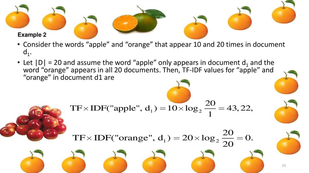
Example 2
• Consider the words “apple” and “orange” that appear 10 and 20 times in document
d1.
• Let |D| = 20 and assume the word “apple” only appears in document d1 and the
word “orange” appears in all 20 documents. Then, TF-IDF values for “apple” and
“orange” in document d1 are
20
TF IDF("apple", d1 ) 10 log 2
43, 22,
1
20
TF IDF("orange", d1 ) 20 log 2
0.
20
25

26. Consider the following three documents:

Example 3
• d1= “social media mining”
• d2= “social media data”
• d3= “financial market data”
• The tf values are as follows: :
social
media
mining
data
financial
market
d1
d2
d3
26

27. Consider the following three documents:

Example 3
• d1= “social media mining”
• d2= “social media data”
• d3= “financial market data”
• The TF values are as follows: :
social
d1
d2
d3
1
1
0
media
1
1
0
mining
1
0
0
data
0
1
1
financial
0
0
1
market
0
0
1
27

28. The IDF values are

3
IDF("social") log 2
0, 584,
2
3
IDF("media") log 2
0, 584,
2
3
IDF("mining") log 2 1, 584,
1
3
IDF("data") log 2
0, 584,
2
3
IDF("financial") log 2 1, 584,
1
3
IDF("market") log 2 1, 584.
1
28

29. The TF-IDF values can be computed by multiplying TF values with the IDF values:

• d1= “social media mining”
• d2= “social media data”
• d3= “financial market data”
d1
d2
d3
social
media
mining
data
financial
market
0,584
0,584
0
0,584
0,584
0
1,584
0
0
0
0,584
0,584
0
0
1,584
0
0
1,584
After vectorization, documents are converted to vectors, and common data mining algorithms can be applied.
However, before that can occur, the quality of data needs to be verified.
29

30. Item Similarity Methods

• Information Retrieval Techniques
Item attributes correspond to word occurrences in item descriptions
yij TFij IDFj, TFij – term frequency: frequency of word yj occurring in the
description of item si; IDFj – inverse document frequency: inverse of the frequency of
word yj occurring in descriptions of all items.
• Content-based profile vi of user ci constructed by aggregating profiles of
items ci has experienced
rˆij score ( v i , y j )
rˆij cos( v i , y j )
vi y j
|| v i ||2 || y j ||2

31. Content-Based kNN Method

• Each item is defined by its content C.
• Content is application-specific, e.g., restaurants vs. music
• Content C is represented as a vector Ĉ=(c1, c2,…, cd)
• E.g., as a TF-IDF vector in the previous case
• Content-based kNN method:
• Assume user also rated n items (r1, r2, …, rn).
• Then for n known item/rating pairs (Ĉ1, r1 ), (Ĉ2, r2), …, (Ĉn, rn) and a new
item Ĉ, estimate its rating r as a weighted average of Ĉ’s k nearest
neighbors, where the distance between two items dist(Ĉ, Ĉi) can be
defined as cos(Ĉ, Ĉi).

32. Item-Based Collaborative Filtering

• Same rij estimation as for the user-based but use item-to-item sim(i, i’) instead
of user-to-user similarity
• Used by Amazon 15 years ago [Linden03]
• Compute item-to-item similarity offline [Linden03]:
For each item i in the catalog
For each user u in Purchased(u, i)
For each item i' in Purchased(u, i’)
Record items i and i' as CoPurchased(i, i’, u)
Compute sim(i, i') based on CoPurchased(i, i’, u)
• Store {u: Purchased(u,i)} & {i: Purchased(u,i)} as lists
A. Tuzhilin

33. Association-Rule-Based CF

Another example of CF heuristic
Assume user A had transaction T with items I = (i1, i2, …, ik).
Q: Which other items should A be recommended?
Step 1 (offline): find the association rules X Y with support and confidence thresholds of
( , ) respectively
Step 2 (online):
a. Find all the rules X Y fired by A’s transaction T
Rules where X is in I
b. Take union of Y’s items not in I across all the fired rules
Remove duplicates: select items with largest confidence
c. Sort them by the confidence levels of their fired rules
d. Recommend to A the top N items in the sorted list.

34. Association-Rule-Based CF: Supermarket Purchases

User A bought I = (Bread, Butter, Fish)
Q: What else to recommend to A?
Step 1: find rules X Y with support and conf >
(25%,60%) respectively
Example: Bread, Butter Milk (s=2/7=29%,
c=2/3=67%)
Step 2:
a. This rule is fired by A’s transaction
b. Thus, add Milk to the list (c=67%)
c. Do the same for all other rules fired by A’s
transaction
d. Recommend Milk to A if Milk makes the
top-N list with c = 67%

35. Hybrid: Combining Other Methods

• The hybrid approach can combine two
or more methods to gain better
performance results.
• Types of combination:
• Weighted combination of the
recommender scores
• Switching between recommenders
depending on the situation
• Cascade: one system refines
recommendations of another
• Mixed: several recommender results
presented together
Example:
Source: Dataconomy

36. Performance Evaluation of RSes

Importance of Right Metrics
• There are measures and… measures!
• Assume you improved the RMSE of Netflix by 10%. So what?
• What do you really want to measure in RSes?
• Economic value/impact of recommendations
• Examples: increase in sales/profits, customer loyalty/churn, conversion
rates,…
• Need live experiments with customers (A/B testing) to measure true
performance of RSes

37. Evaluation Paradigms

• User studies
• Online evaluations (A/B tests)
• Offline evaluation with observational data
• Long-term goals vs. short-term proxies
• Combining the paradigms: offline and online evaluations

38. Example of A/B Testing

• Online University: a RS recommends remedial learning materials to the
students who have “holes” in their studies
• Applied this Recommender System to
42 different courses from CS, Business and General Studies
over 3 semesters of 9 weeks each
910 students from all over the world
1514 enrollments in total (i.e., 1514 student/course pairs).
• Goal: show that this RS “works:” students following the advice perform better
than the control group.

39. Accuracy-Based Metrics

• For Prediction
• RMSE and MAE
• For Classification
• Precision: percentage of good recommendations among all the recommended items
• Recall: percentage of items predicted as good among all the actually good items
• F-measure: 2*Prec*Recall/(Prec + Recall)
• For Ranking
• Discounted cumulative gain (DCG)
• Where reli is relevance of recommended item in position i.

40. Netflix Prize Competition

• Competition for the best algorithm to predict user ratings for films based on prior
ratings
• Data: training dataset of 100,480,507 ratings over 7 years
• 480,189 users and 17,770 movies
• Task: improve RMSE by 10% over Netflix’s own algorithm
• Prize: $1,000,000
• Starting date: October 2, 2006
• The size: 20,000+ teams from over 150 countries registered; 2,000 teams submitted
over 13,000 prediction sets (June 2007)
• Results: 2 teams reached the 10% goal on July 26, 2009:
• BelKor Pragmatic Chaos (7 ppl) and Ensemble (20 ppl)
• RMSE was improved from 0.9514 to 0.8567 (over almost 3 years!)
• $1M Prize awarded to BelKor Pragmatic Chaos on 9/18/2009

41. Test Set Results (RMSE)

• The Ensemble:
0.856714
• BellKor’s Pragmatic Theory: 0.856704
• Both scores round to
0.8567
• Tie breaker is submission date/time
41

42. What Netflix Prize Winners Done

• Development of new and scalable methods, MF being the most
prominent one
• Some Collaborative Filtering methods used in the competition:
k-NN
Matrix Factorization (with different “flavors”)
Regression on Similarity
Time Dependence Models
Restricted Boltzmann Machine
• (Re-)discovered the power of ensemble (hybrid) methods (“blending”)

43. Netflix Competition: The End of an Era

Netflix Prize Competition:
• Completed not only the 2D, but also the 3MR paradigm:
• 3 matrices Ratings, Users and Items
• Utility of an item to a user revealed by a single rating
• Recommendations of individual items provided to individual users
• Developed more efficient solutions to a well-studied problem [AT05]
• Scalability was novel: no 100M ratings dataset before

44. Thinking Outside of the 3MR Box

• The 3MR paradigm worked well for Netflix. But what about other
applications?
Music, e.g. Pandora and Spotify?
Social networks, e.g., LinkedIn and Facebook
News and other reading materials, e.g., Google News
Restaurants, e.g., Yelp
Clothes, e.g. Stitch Fix
It is hard to use just CF, content-based or hybrid methods in these
1G (3MR)
applications.
2G
performance
time

45. Context-Aware Recommender Systems (CARS)

• Recommend a vacation
• Winter vs. summer
• Recommend a movie
• To a student who wants to see it on Saturday night with his girlfriend in a
movie theater
• Recommendations depend on the context
• Need to know not only what to recommend to whom, but also under what
circumstances
• Context: Additional information (besides Users and Items) that is relevant to
recommendations

46. What is Context in Recommender Systems

• A multifaceted concept: 150 (!) definitions from various
disciplines (Bazire&Brezillon 05)
• One approach: Context can be defined with contextual
variables C = C1 … Cn, e.g.,
• C = PurchaseContext TemporalContext
• c = (work, weekend), i.e., work-related purchases on a
weekend
• Contextual variables Ci have a tree structure

47. Context-Aware Recommendation Problem

• Data in context-aware recommender systems (CARS)
• Rating information: <user, item, rating, context>
• In addition to information about items and users, also
may have information about context
• Problem: how to use context to estimate unknown ratings?

48. How to Use Context in Recommender Systems [AT10]

Context can be used in the following stages of the recommendation process:
• Contextual pre-filtering
• Contextual information drives data selection for that context
• Ratings are predicted using a traditional recommender on the selected data
• Contextual post-filtering
• Ratings predicted on the whole data using traditional recommender
• The contextual information is used to adjust (“contextualize”) the resulting set of
recommendations
• Contextual modeling
• Contextual information is used directly in the modeling technique as a part of
rating estimation

49. Paradigms for Incorporating Context in Recommender Systems [AT08]

Contextual Post-Filtering
Contextual Pre-Filtering
Data
U I C R
Contextual Modeling
Data
U I C R
Data
U I C R
2D Recommender
U I R
MD Recommender
U I C R
c
Contextualized Data
U I R
2D Recommender
U I R
Recommendations
i1, i2, i3, …
c
c
Contextual
Recommendations
i1, i2, i3, …
Contextual
Recommendations
i1, i2, i3, …
Contextual
Recommendations
i1, i2, i3, …

50. Multidimensional Recommender Systems

Traditional 2D Matrix
3
Un
10
…
Im
…
5
…
I1
I2
…
ITEMS
U1
USERS
U2
…
7
…
…
…
Multidimensional (OLAP-based) cube
8
6
Users
Problem: how to estimate ratings on
this cube?
Time
Items

51. Mobile Recommender Systems

• A special case of CARS
• Very different from traditional RSes
• Spatial context
• Temporal context
• Trace data (sequences of locations &
events)
• Less rating-dependent

52. Route Recommendations for Taxi Drivers (based on [Ge et al 2010])

• Goal: recommend travel routes to taxi (or Uber) drivers to improve
their economic performance
• Defining features:
• Input data: driving/location traces
• Recommendation: a driving route (space/time)
• Performance metric: economics-based, e.g.,
• Revenue per time unit
• Minimize idle/empty driving time
• Example: recommend best driving routes to pick passengers to
minimize empty driving
• Challenge: combinatorial explosion!

53. Key Ideas Behind the Solution

• Need to model/represent driving routes
• Finite set of popular/historical “pick up points”
• Cluster them into pickup hubs (use of clustering techniques)
• Route recommendation: sequence of pickup hubs
• Compute expected “empty” travel distances
• Performance measure: Potential Travel Distance
• Leverage prior driving patterns of experienced taxi drivers to recommend
“good” routes
• Less experienced drivers should follow the driving patterns of more
experienced drivers (“collaborative” approach)
• Technical details in [Ge et al. 2010]

54. Results of a Study

• Data on 500 taxis in SF driving over 30 days
• “Successful” drivers: over 230 driving hours and 0.5 occupancy rates; 20 such drivers
(the “role models”)
• Focus on 2 time periods: 2 – 3pm & 6 – 7pm
• Computed 636 and 400 historical pickup points for these 2 periods based on 20 good
drivers
• Computed driving distances between these points using Google Map API
• Computed 10 clusters for 636 & 400 pickup points
• Construct an optimal route for a new driver at that time (based on these clusters)
and recommend it to him/her.
(DL)

55. Why DL for RSes?

ImageNet challenge error rates (red line = human performance)

56. DL for Vehicle Recommendations

• Using deep learning to improve vehicle suggestions, we have two
basic goals:
• Increase the relevance of recommendations
• Provide them in a scalable way
[M. Kurovski]

57. Preference Prediction Model

The overall network consists of three
subnetworks: UserNet, ItemNet and
RankNet.
These networks are combined and
trained jointly. Afterwards, we split
them to present an overall
architecture capable of serving the
recommendations in production.

58. Candidate Generation

• To quickly find candidates that are likely to be relevant for a user, we
use approximate nearest neighbor search. Starting with a user
embedding as query, we can efficiently fetch the T closest items for a
specific distance metric, e.g. cosine or Euclidean distance.
• There are many implementations, including Locally Optimized Product
Quantizations (LOPQ) from Yahoo or Approximate Nearest Neighbor
Oh Yeah (ANNOY) provided by Erik Bernhardsson from Spotify.
[M. Kurovski]

59. Ranking

• For T item candidates
for our user, we can
use the RankNet to
score each candidate.
• Finally, we sort the
candidates by
decreasing score and
take the top k most
promising ones.
• These items are then
provided as
recommendations [M. Kurovski]

60. Deep content-based music recommendation

Pioneer work
from Spotify also
uses CNNs to
extract audio
features from
music tracks.
The content
features could
then used to
cluster similar
tracks and to
produce
personalized
playlists.
https://papers.nips.cc/paper/5004-deep-content-based-music-recommendation.pdf

61. Is deeper better?

For image classification deeper models
with hundreds of layers and novel
architecture shave shown impressive
improvements reducing the
classification error more that 24
percentage points in the last few years.
What about DL for RecSys? are such
improvement in recommendation
performance possible?
https://medium.com/@libreai/a-glimpse-into-deep-learning-for-recommender-systems-d66ae0681775

62. Unexpected & Serendipitous RSes

Unexpected & Serendipitous RSes

63.

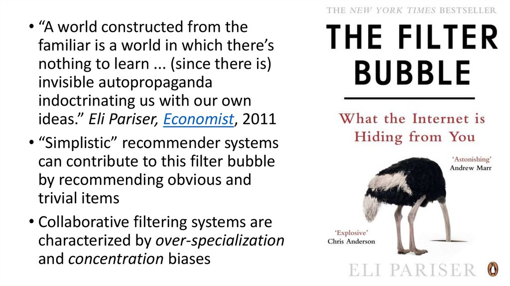
• “A world constructed from the
familiar is a world in which there’s
nothing to learn ... (since there is)
invisible autopropaganda
indoctrinating us with our own
ideas.” Eli Pariser, Economist, 2011
• “Simplistic” recommender systems
can contribute to this filter bubble
by recommending obvious and
trivial items
• Collaborative filtering systems are
characterized by over-specialization
and concentration biases

64. The Filter Bubble Example

Problem with accuracy: can lead to
boring recommendations

65. Serendipity and Unexpectedness: Breaking out of the Filter Bubble

Serendipity: Recommendations of novel items liked by the user that he/she would
not discover autonomously (accidental discovery)
Unexpectedness: tell me something surprising that goes against my
expectations

66. Definition of Unexpectedness

• “If you do not expect it, you will not find the unexpected, for it is hard to
find and difficult.” - Heraclitus of Ephesus, 544-484 B.C.
• Idea:
• Define user expectations
• Identify those items that depart from those expectations
• Recommend high quality and unexpected items to the user

67. Examples of Unexpected Recommendations

User Profile
Recommendations

68. Expected Recommendations

• Expectation set of a user: a finite collection of items that the user
considers as familiar/known/expected.
• Multiple ways to define this set.
Examples of sets of user expectations
Domain
Movies
Books
Mechanism
Method
Past Transactions
Explicit Ratings
Domain Knowledge
Set of Rules
Past Transactions
Implicit Ratings
Domain Knowledge
Related Items
Data Mining
Association Rules

69. Operationalization of Unexpectedness

70. Utility of Recommendations

71. Unexpectedness and the Long Tail

• The “rich gets richer” problem of RSes (a.k.a. the “blockbuster”
phenomenon)
• Many RS algorithms tend to recommend popular items (from the “Head” of the
Long Tail distribution), thus reinforcing the “filter bubble” phenomenon…
• Whereas the real “action” is in the Long Tail
• Unexpected recommendations are more from the Long Tail because they
• produce more diverse recommendations
• do not recommend expected items from the Head

72. Tomorrow: Deep Learning for Human-Computer Interaction

Tomorrow: Deep Learning for HumanComputer Interaction

73.

Thank you.
Inna Skarga-Bandurova
Computer Science and Engineering Depatrment
V. Dahl East Ukrainian National University
[email protected]