


")
")
")
")
")
")
")
")


 Экономика
Похожие презентации:


Forecasting Free Cash Flow of an Industrial Enterprise Using Fuzzy Set Tools
1. Forecasting Free Cash Flow of an Industrial Enterprise Using Fuzzy Set Tools
Higher School of EconomicsNational Research University
St Petersburg Campus
Forecasting Free Cash Flow of an Industrial Enterprise
Using Fuzzy Set Tools
Elena Tkachenko
Saint Petersburg State University of Economics
Elena Rogova
National Research University Higher School of Economics
Daria Koval
Saint Petersburg State University of Economics
2. Motivation
• The problem of forecasting companies’ cash flows is important in thegrowing uncertainty of the business environment
• It is also discussed in the literature (Kaplan, Ruback, 1995; Fridson,
Alvarez, 2009; Cheng, Czernkowski, 2010; Pae, Yoon, 2012; Ruppert, 2017)
• One of the main objectives of forecasting is to enhance the enterprise's
ability to react to changes of the external environment that might affect
the performance
3. Methods of Cash Flow Forecasting
FCFF EBIT (1 Tax Rate) DA NWC CapexMethod
Applicability
Linear trend
Analytic formulas:
polynomial;
logarithmic;
exponential;
geometrical
Used in the context of a company’s progressive development
Requires regularity, or rhythmicity, unrelated to seasonality:
when using cyclical indicators;
when forecasting indicators that, after a period of growth/drop, reach a
certain level of stability;
when a linear trend having clearly defined curvature is present; or
at an appropriate stage of an enterprise’s life cycle.
The Chained Percentage
Seasonal fluctuation is required
Ratio Method
Correlation
with Proven relation with the macroeconomic situation is required
macroeconomic indicators
Forecasting is available for a short period
The Brown Method
The Holt-Winters
Method
Partitioning of seasonal fluctuation sand main trend to track,
analyze and evaluate their mutual influence
4. Revenues as a Key Element to be Forecasted
Revenues generated by various centers of financial responsibilities and revenues
from varying focus areas generated under the influence of different factors may
be forecasted using various methods
The resulting forecast is based on data obtained on all levels of research starting
with the macroeconomic level and down to the level of enterprise. At this stage,
variants of macroeconomic and microeconomic dynamics are compared, and the
enterprise's response scenarios to changes of the internal and external
environments are developed.
Due to the modern volatility of global and national economies, the significance
of forecasting, in general, and enterprise revenue forecasting, in particular (being
part of the budgeting process) is greater than ever.
The models mentioned above are limited, to some extent, and often, their use
does not make it possible to obtain the desired result due to certain inherent
risks and errors.
5. Fuzzy Time Series (1)
• When discussing fuzzy time series {Ỹ(t)}, it should be noted thatsuch a series includes a number of fuzzy sets Xt, where t = 1, 2, …
• In this case, we used the assumption that the components of the
series Xt have linguistic values, and Ỹ(t) is a fuzzy function with
argument t which values have fuzzy verbal variables “high”,
“average”, “low”, etc.
• The use of logical-linguistic variables makes it possible to take into
account qualitative factors that enable to recognize the uncertainty
• Empirical data of the time series {Y(t)} must be designated. These
are selected with account to the objective of study (revenue of the
enterprise, per-capita income, GDP, etc.)
6. Fuzzy Time Series (2)
By studying a time series in a fuzzy dynamic environment one is able to formulate a fuzzy
function Ỹ(t) with argument t, within the universal set of U, having the set of values designated
as fuzzy ranges Xt and membership function µXt(ui). Thus, (2) is obtained:
Xt = {µX t (ui)/ui},
where Xt is fuzzy range; µXt(ui) is membership function; and t is argument of the function; and the
following conditions are met:
ui∈ U; µXt (ui) ∈[0, 1].
The conditions considered signify that every point within the interval of ui will be a member of
the set Xt and have the degree of membership of:
µXt (ui) = µi (t),
where µi (t) are given numbers, i=; 1, t = [1, 2,…].
Thus, the complete set or range of number axis will appear as:
U = (u1, u2, …, um),
where ,ui, i = 1,m.
• The fuzzy set of X of the universal set of U may be defined as:
X = {(μx(u1)/u2), (μx(u1)/u2), …, (μx(um)/um)},
where μx(ui) is the membership function which puts its elements ui as a set of real numbers within
the segment of [0, 1] indicating the degree of membership of elements ui in the set of X, μx(ui)∈
[0, 1];“/” designates the membership of the value μx in the element um.
7. Stages for forecasting with Fussy Time Series (1)
Stage 1• The process of defining the complete U set.
Stage 2
• Dividing the U set into several intervals of equal length.
Stage 3
• Distinguishing a set of fuzzy sets within the universal U set.
Stage 4
• Converting precise numerical values of the time series into
fuzzy values
Stage 5
• Forecasting time series values in terms of fuzzy logic
Stage 6
• Converting the fuzzy values of the time series into precise values.
8. Stages for forecasting with Fuzzy Time Series (2)
• At the first stage, the boundaries of the time series aredefined, and the indicators necessary to solve the
forecasting problem are selected. To define the
universal U set, increment of the considered indicator
of the time series throughout the time interval must be
determined. It should be noted that boundaries of the
universal set U coincide with the maximum and
minimum values of the indicator increment, however,
at the following stages of the forecasting process these
boundaries may be expanded for the ease of
calculation.
• At the second stage, the defined universal U set is
divided into intervals having equal length.
9. Stages for forecasting with Fuzzy Time Series (3)
• At the third stage of the analysis, a set of fuzzy sets shall be identifiedwithin the previously determined universal U set. For this purpose, logicallinguistic variables shall be introduced and appropriate values of these
variables determined. In general terms, these variables may be as follows:
• very low level of increment of the forecasted indicator (VLLIFI);
• low level of increment of the forecasted indicator (LLIFI);
• average level of increment of the forecasted indicator (ALIFI);
• stationary level of increment of the forecasted indicator (SLIFI);
• normal level of increment of the forecasted indicator (NLIFI);
• high level of increment of the forecasted indicator (HLIFI); and
• very high level of increment of the forecasted indicator (VHLIFI).
10. Stages for forecasting with Fuzzy Time Series (4)
• In order to define the fuzzy set Аi within the universal U set, membershipfunction shall be used.
• Thus, by consistently adopting the average value ui of middle point of the
intervals as the value of variable V we can develop the following
representation of fuzzy sets:
• А1 = {(/u1), (/u2), (/u3), (/u4), (/u5), (/u6), (/u7)}
• А2 = {(/u1), (/u2), (/u3), (/u4), (/u5), (/u6), (/u7)}
• А3 = {(/u1), (/u2), (/u3), (/u4), (/u5), (/u6), (/u7)}
• А4 = {(/u1), (/u2), (/u3), (/u4), (/u5), (/u6), (/u7)}
• А5 = {(/u1), (/u2), (/u3), (/u4), (/u5), (/u6), (/u7)}
• А6 = {(/u1), (/u2), (/u3), (/u4), (/ u5), (/u6), (/u7)}
• А7 = {(/u1), (/u2), (/u3), (/u4), (/ u5), (/u6), (/u7)}.
11. Stages for forecasting with Fuzzy Time Series (5)
At the fourth stage, conversion of numerical values of increment of the forecasted indicator
into fuzzy values is performed. At this stage, qualitative representations of the dynamics of
increment of the forecasted indicator is accounted for in the form of fussy sets
At the fifth stage, forecasting of the studied indicator is done using fuzzy logic symbols.
To forecast the value of increment of the studied indicator for the period of t resulting in the
fuzzy set of F(t)), fuzzy relation matrix R(t) must be calculated. This matrix is determined by
intersecting the matrix of fuzzy increment of the studied indicator N(t) for the period of (t-1)
and the matrix of fuzzy increments of the studied indicator S(t) for the periods of (t-2), (t-3),
(t-4), (t-5), (t-+).Therefore:
In this case F(t) = [max(r11, r21, …, ri1) max(r12, r22, …, ri2) … max(r1j, r2j, …,rij)].
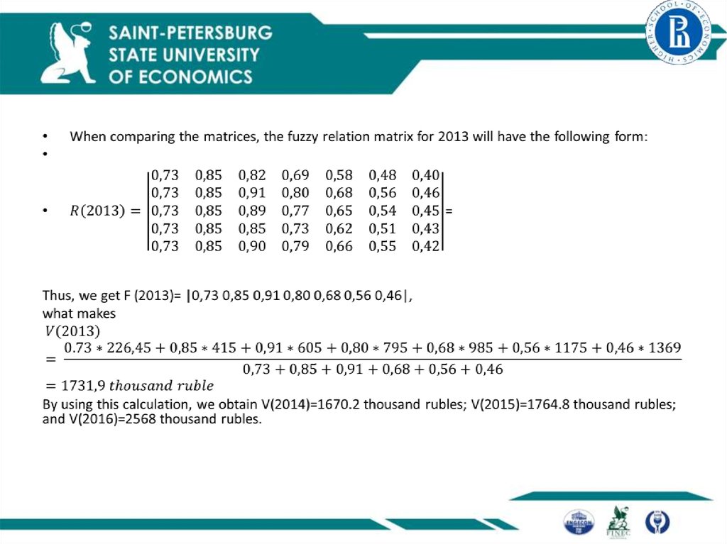
12. Stages for forecasting with Fuzzy Time Series (6)
• At the sixth stage, conversion of fuzzy values of increment of thestudied indicator into precise values is performed. For
implementing this, we use a formula:
• where µt(ui) are the values of membership function for the
considered year and uсрi are coordinates of points dividing intervals
of equal length into equal parts ui that belong to the universal U
set.
• In order to obtain the value of the forecasted indicator, the value of
the forecasted increment must be added to its value for the last
period.
13. Using the Method for Cash Flows Predicting
Year2009
2010
2011
2012
2013
2014
2015
2016
Revenue in thousands rubles
358987
396781
429187
498745
517896
629800
690494
693203
Revenue gain in thousands rubles
37794
32406
69558
19151
11904
60694
2709
According to the proposed method, boundaries of the universal set U shall
correspond to the maximum and minimum value of increment for the considered
year, what makes U = [2700; 69700]. Let us divide the defined boundaries into
seven equal intervals having the length of 9570 that will be represented as: u1=
[2700, 12270]; u2= [12270, 218840]; u3= [21840,31410]; u4=[31410, 40980]; u5 =
[40980, 50550]; u6 = [50550, 60120]; u7 = [60120, 69700], then = 7485; = 17055;
14. Variables and Their Values
very low level of revenue gain (VLLRG);
low level of revenue gain (LLRG);
average level of revenue gain (ALRG);
stationary level of revenue gain (SLRG);
normal level of revenue gain (NLRG);
high level of revenue gain (HLRG); and
very high level of revenue gain (VHLRG).
15. Conversion of Fuzzy Sets
Let us define a fuzzy set Аi within the universal set U according to the formula discussedabove where c=0.0001, and we will obtain a representation of fuzzy sets:
А1 = {(1/u1), (0,97/u2), (0,87/u3), (0,75/u4), (0,63/u5), (0,53/u6), (0,43/u7)}
А2 = {(0,97/u1), (1/u2), (0,97/u3), (0,87/u4), (0,75/u5), (0,63/u6), (0,53/u7)}
А3 = {(0,87/u1), (0,97/u2), (1/u3), (0,97/u4), (0,87/u5), (0,75/u6), (0,63/u7)}
А4 = {(0,75/u1), (0,87/u2), (0,97/u3), (1/u4), (0,97/u5), (0,87/u6), (0,75/u7)}
А5 = {(0,63/u1), (0,75/u2), (0,87/u3), (0,97/u4), (1/u5), (0,97/u6), (0,87/u7)}
А6 = {(0,53/u1), (0,63/u2), (0,75/u3), (0,87/u4), (0,97/ u5), (1/u6), (0,97/u7)}
А7 = {(0,43/u1), (0,53/u2), (0,63/u3), (0,75/u4), (0,87/ u5), (0,97/u6),(1/u7)}.
Revenue
Gain
37794
а1 = {(1/u ), (0,95/u ), (0,85/u ), (0,73/u ), (0,62/u ), (0,51/u ), (0,42/u )}
32406
а2 = {(1/u ), (0,98/u ), (0,90/u ), (0,79/u ), (0,66/u ), (0,55/u ), (0,45/u )}
69558
19151
11904
60694
2709
а3 = {(0,73/u ), (0,85/u ), (0,95/u ), (1/u ), (0,97/u ), (0,89/u ), (0,77/u )}
а4 = {(0,83/u ), (0,97/u ), (1/u ), (0,95/u ), (0,85/u ), (0,73/u ), (0,61/u )}
а5 = {(0,85/u ), (0,94/u ), (1/u ), (0,98/u ), (0,90/u ), (0,78/u ), (0,66/u )}
а6 = {(0,62/u ), (0,74/u ), (0,86/u ), (0,96/u ), (1/u ), (0,98/u ), (0,88/u )}
а7 = {(0,40/u ), (0,48/u ), (0,58/u ), (0,70/u ), (0,82/u ), (0,93/u ), (1/u )}
Conversion into Fuzzy Sets
16.
17. Revenues Forecasting
Forecasting MethodAverage
Approximation
Error in %
2013
2014
2015
2016
Precise Time Series
Method
518,743.5
630,676.0
690,013.6
69,314.7
19.72
Fuzzy Time Series
Method
519,627.9
631,470.2
692,258.8
695,771
5.98
18. Conclusion
• The proposed forecasting method based on fuzzy sets is an addition to theexisting quantitative methods of forecasting. Application of this method
promotes the reduction of approximation error below the level of
reduction achieved when forecasting using statistical methods. This
indicates that this model has practical significance and enhances the
accuracy of forecast.
• Application of forecasting using the fuzzy set method and linear model
demonstrated that the fuzzy set method made it possible to bring average
approximation error down by 13.7%.
• This allows for the conclusion that forecast accuracy is increased