Dynamic Programming. Lec 10

1. ADVANCED ALGORITHMS & DATA STRUCTURES

ADVANCED ALGORITHMS &
DATA STRUCTURES
Lecture-10
Dynamic programming
Lecturer: Karimzhan Nurlan Berlibekuly
[email protected]

2. Dynamic Programming

3. Dynamic Programming

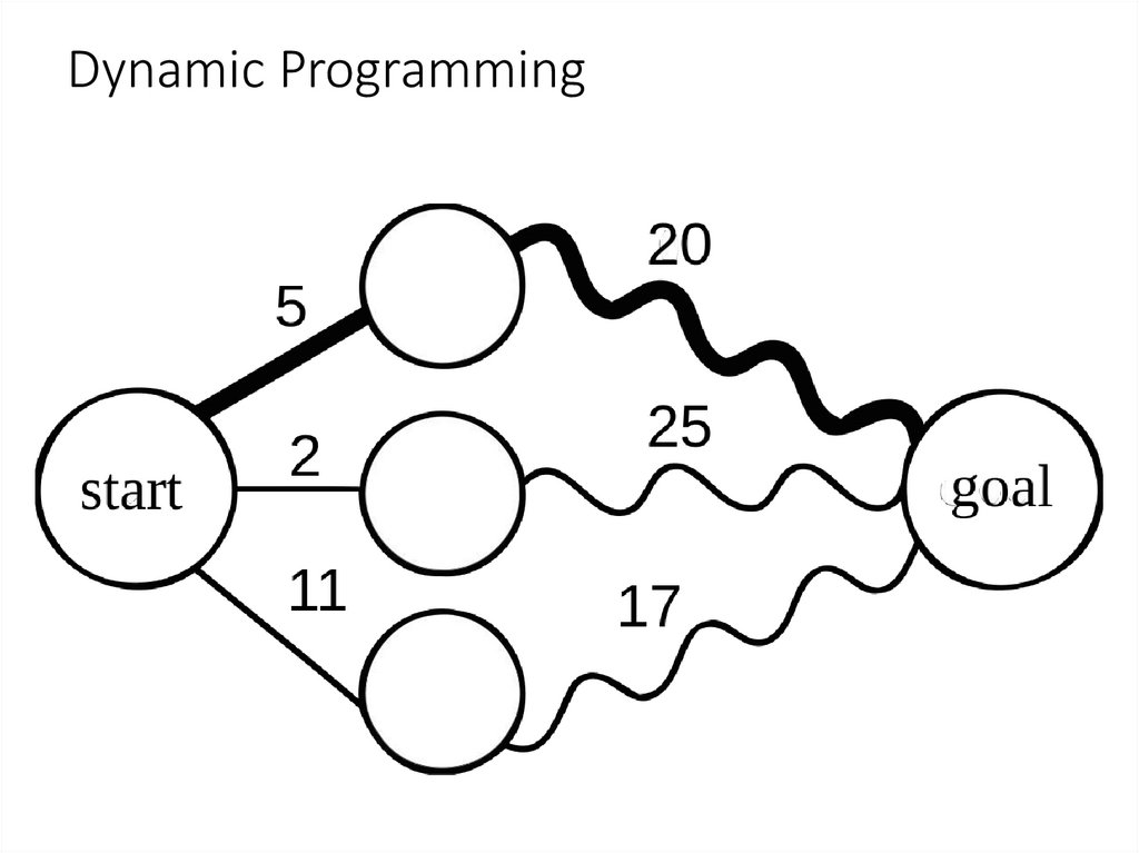
Dynamic Programming is mainly an optimization over
plain recursion. Wherever we see a recursive solution
that has repeated calls for same inputs, we can optimize
it using Dynamic Programming.
The idea is to simply store the results of subproblems, so
that we do not have to re-compute them when needed
later. This simple optimization reduces time complexities
from exponential to polynomial.

4. Dynamic Programming

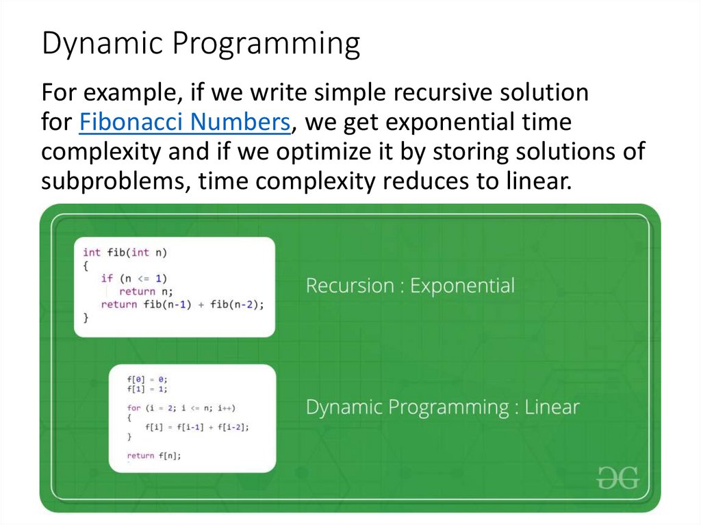
For example, if we write simple recursive solution
for Fibonacci Numbers, we get exponential time
complexity and if we optimize it by storing solutions of
subproblems, time complexity reduces to linear.

5. Dynamic Programming 1 Introduction

In this lecture we introduce dynamic programming,
which is a high-level computational thinking concept
rather than a concrete algorithm. Perhaps a more
descriptive title for the lecture would be sharing,
because dynamic programming is about sharing
computation. We know that sharing of space is also
crucial: binary decision diagrams in which subtrees are
shared are (in practice) much more efficient than binary
decision trees in which there is no sharing.

6. Dynamic Programming

In order to apply dynamic programming, we generally
look for the following conditions:
1. The optimal solutions to a problem is composed of
optimal solutions to subproblems, and
2. if there are several optimal solutions, we don’t care
which one we get.

7. 2 Fibonacci Numbers

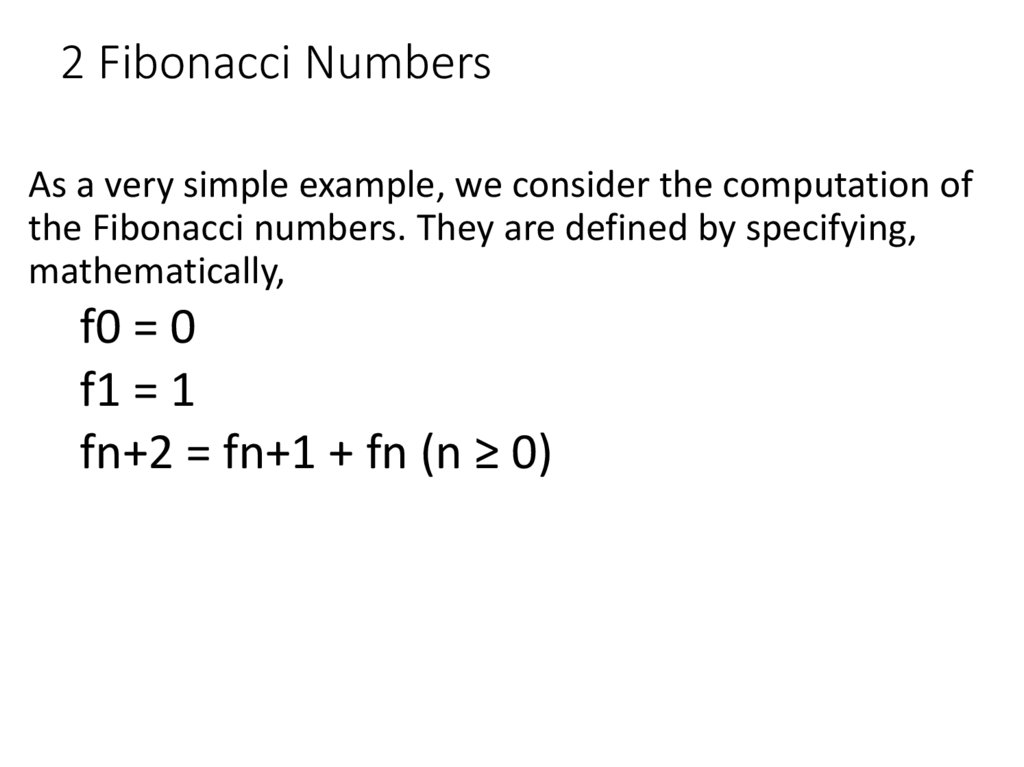
As a very simple example, we consider the computation of
the Fibonacci numbers. They are defined by specifying,
mathematically,
f0 = 0
f1 = 1
fn+2 = fn+1 + fn (n ≥ 0)

8. 2 Fibonacci Numbers

A direct (and very inefficient) implementation is a recursive
function
int fib0(int n) {
REQUIRES(n >= 0);
if (n == 0) return 0;
else if (n == 1) return 1;
else return fib0(n-1) + fib0(n-2);
}
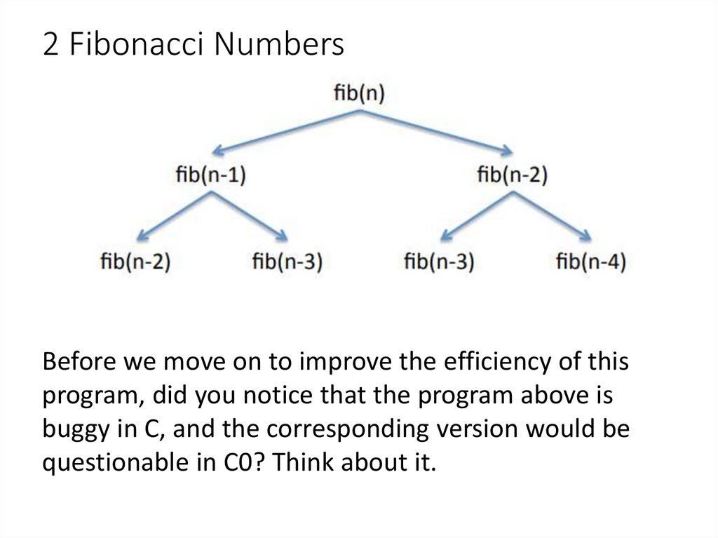
When we draw the top part of a tree of the recursive calls
that have to be made, we notice that values are computed
multiple times.

9. 2 Fibonacci Numbers

Before we move on to improve the efficiency of this
program, did you notice that the program above is
buggy in C, and the corresponding version would be
questionable in C0? Think about it.

10. 2 Fibonacci Numbers

The problem is that addition can overflow. In C, the result
is undefined, and arbitrary behavior by the code would
be acceptable. In C0 the result would be defined, but it
would be the result of computing modulo 2^32 which
could be clearly the wrong answer. We can fix this by
explicitly checking for overflow.

11. 2 Fibonacci Numbers

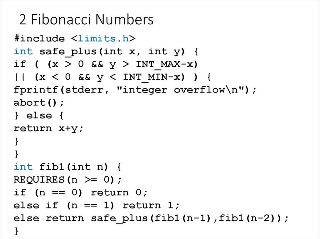
#include <limits.h>
int safe_plus(int x, int y) {
if ( (x > 0 && y > INT_MAX-x)
|| (x < 0 && y < INT_MIN-x) ) {
fprintf(stderr, "integer overflow\n");
abort();
} else {
return x+y;
}
}
int fib1(int n) {
REQUIRES(n >= 0);
if (n == 0) return 0;
else if (n == 1) return 1;
else return safe_plus(fib1(n-1),fib1(n-2));
}

12. 3 Top-Down Dynamic Programming

In top-down dynamic programming we store the values as we
compute them recursively. Then, if we need to compute a value we
just reuse the value if we have computed it already. A characteristic
pattern for top-down dynamic programming is a top-level function
that allocates an array or similar structure to save computed
results, and a recursive function that maintains this array.

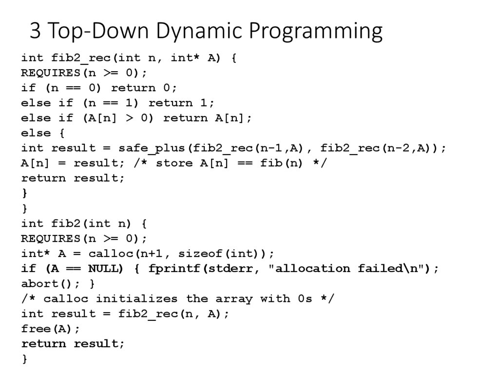
13. 3 Top-Down Dynamic Programming

int fib2_rec(int n, int* A) {
REQUIRES(n >= 0);
if (n == 0) return 0;
else if (n == 1) return 1;
else if (A[n] > 0) return A[n];
else {
int result = safe_plus(fib2_rec(n-1,A), fib2_rec(n-2,A));
A[n] = result; /* store A[n] == fib(n) */
return result;
}
}
int fib2(int n) {
REQUIRES(n >= 0);
int* A = calloc(n+1, sizeof(int));
if (A == NULL) { fprintf(stderr, "allocation failed\n");
abort(); }
/* calloc initializes the array with 0s */
int result = fib2_rec(n, A);
free(A);
return result;
}

14. 3 Top-Down Dynamic Programming

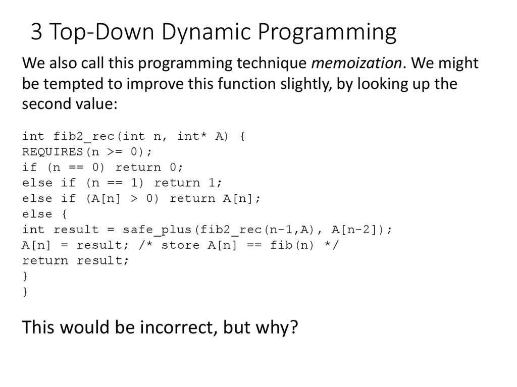
We also call this programming technique memoization. We might
be tempted to improve this function slightly, by looking up the
second value:
int fib2_rec(int n, int* A) {
REQUIRES(n >= 0);
if (n == 0) return 0;
else if (n == 1) return 1;
else if (A[n] > 0) return A[n];
else {
int result = safe_plus(fib2_rec(n-1,A), A[n-2]);
A[n] = result; /* store A[n] == fib(n) */
return result;
}
}
This would be incorrect, but why?

15. 4 Bottom-Up Dynamic Programming

Top-down dynamic programming retains the structure of the
original (inefficient) recursive function. Bottom-up dynamic
programming inverts the order and starts from the bottom of the
recursion, building up the table of values. In bottom-up dynamic
programming, recursion is often profitably replaced by iteration.

16. 4 Bottom-Up Dynamic Programming

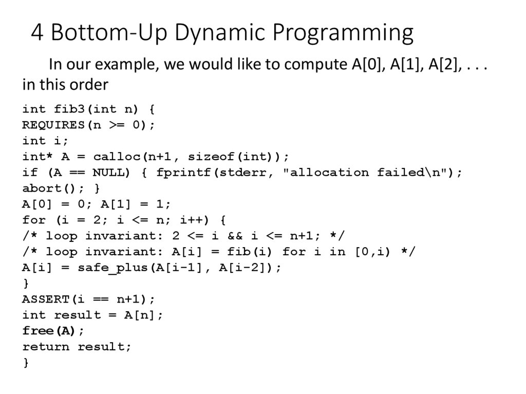
In our example, we would like to compute A[0], A[1], A[2], . . .
in this order
int fib3(int n) {
REQUIRES(n >= 0);
int i;
int* A = calloc(n+1, sizeof(int));
if (A == NULL) { fprintf(stderr, "allocation failed\n");
abort(); }
A[0] = 0; A[1] = 1;
for (i = 2; i <= n; i++) {
/* loop invariant: 2 <= i && i <= n+1; */
/* loop invariant: A[i] = fib(i) for i in [0,i) */
A[i] = safe_plus(A[i-1], A[i-2]);
}
ASSERT(i == n+1);
int result = A[n];
free(A);
return result;
}

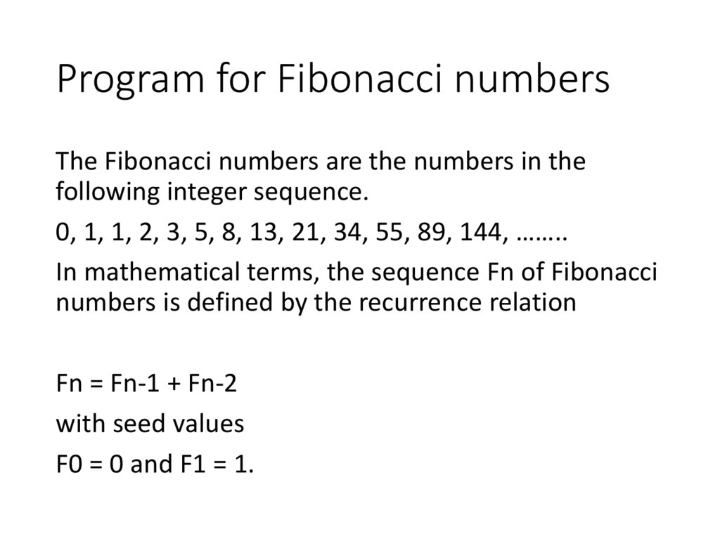
17. Program for Fibonacci numbers

The Fibonacci numbers are the numbers in the
following integer sequence.
0, 1, 1, 2, 3, 5, 8, 13, 21, 34, 55, 89, 144, ……..
In mathematical terms, the sequence Fn of Fibonacci
numbers is defined by the recurrence relation
Fn = Fn-1 + Fn-2
with seed values
F0 = 0 and F1 = 1.

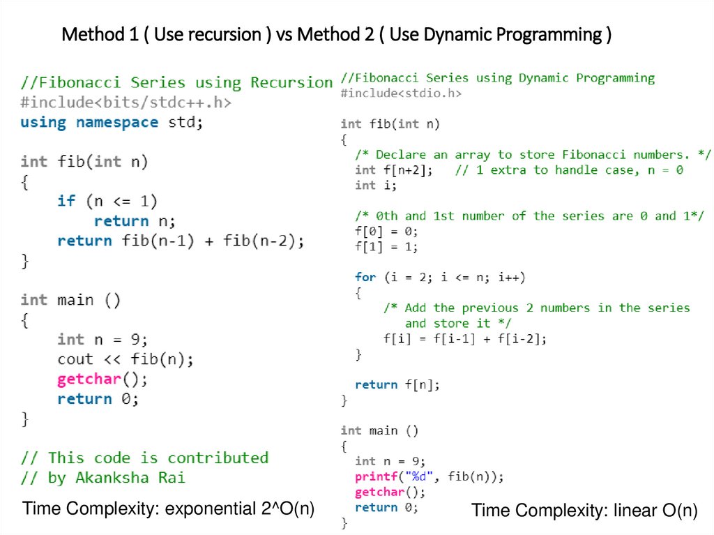
18. Method 1 ( Use recursion ) vs Method 2 ( Use Dynamic Programming )

Time Complexity: exponential 2^O(n)
Time Complexity: linear O(n)

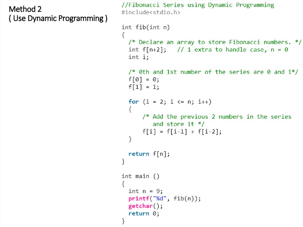
19. Method 2 ( Use Dynamic Programming )

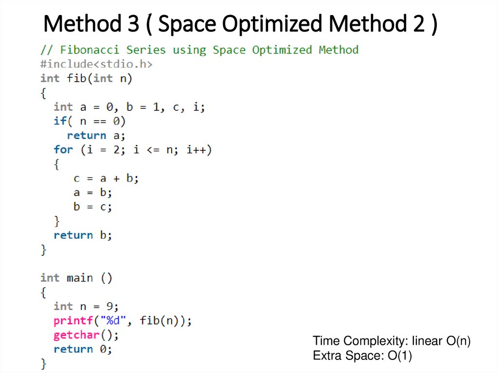
20. Method 3 ( Space Optimized Method 2 )

Time Complexity: linear O(n)
Extra Space: O(1)

21. Method 4 ( Using power of the matrix {{1,1},{1,0}} )

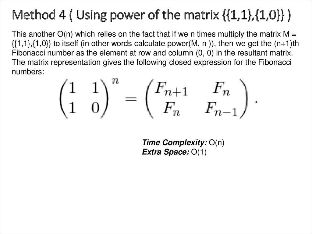
This another O(n) which relies on the fact that if we n times multiply the matrix M =
{{1,1},{1,0}} to itself (in other words calculate power(M, n )), then we get the (n+1)th
Fibonacci number as the element at row and column (0, 0) in the resultant matrix.
The matrix representation gives the following closed expression for the Fibonacci
numbers:
Time Complexity: O(n)
Extra Space: O(1)

22. Method 4 ( Using power of the matrix {{1,1},{1,0}} )

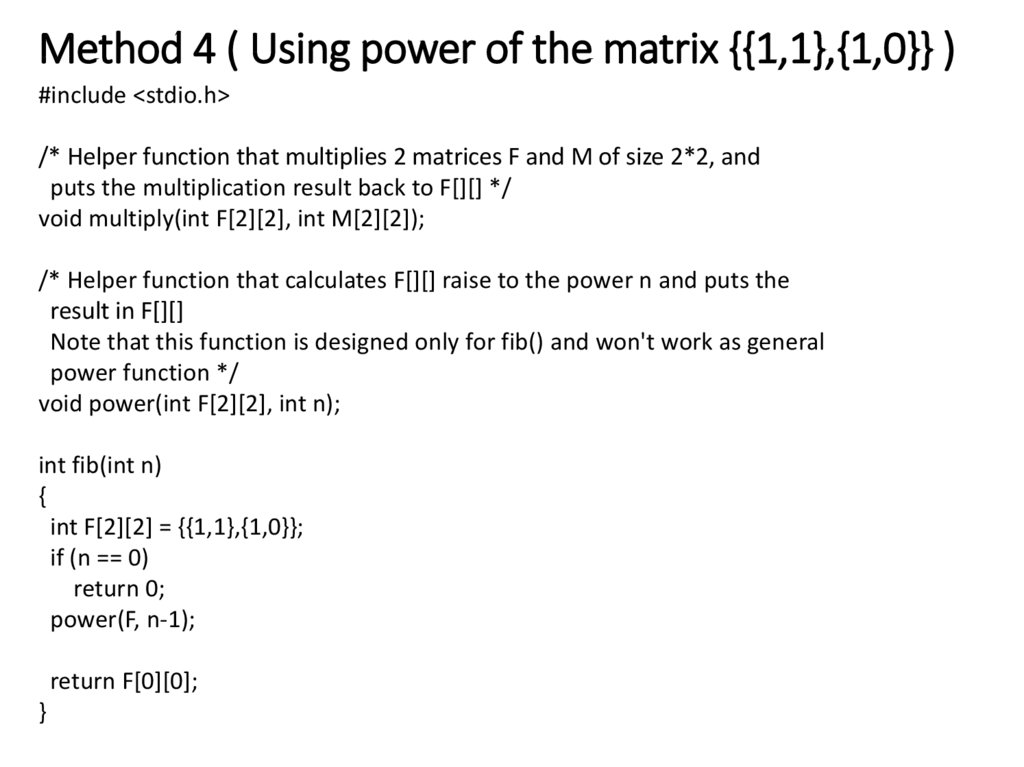
#include <stdio.h>
/* Helper function that multiplies 2 matrices F and M of size 2*2, and
puts the multiplication result back to F[][] */
void multiply(int F[2][2], int M[2][2]);
/* Helper function that calculates F[][] raise to the power n and puts the
result in F[][]
Note that this function is designed only for fib() and won't work as general
power function */
void power(int F[2][2], int n);
int fib(int n)
{
int F[2][2] = {{1,1},{1,0}};
if (n == 0)
return 0;
power(F, n-1);
return F[0][0];
}

23. Method 4 ( Using power of the matrix {{1,1},{1,0}} )

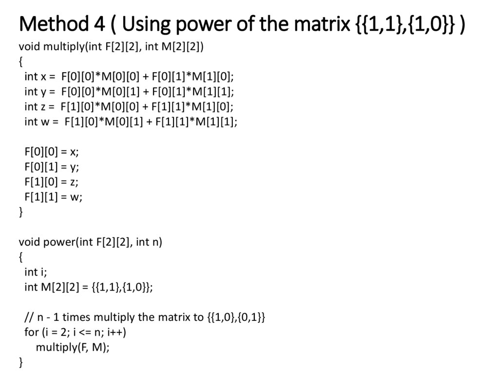
void multiply(int F[2][2], int M[2][2])
{
int x = F[0][0]*M[0][0] + F[0][1]*M[1][0];
int y = F[0][0]*M[0][1] + F[0][1]*M[1][1];
int z = F[1][0]*M[0][0] + F[1][1]*M[1][0];
int w = F[1][0]*M[0][1] + F[1][1]*M[1][1];
F[0][0] = x;
F[0][1] = y;
F[1][0] = z;
F[1][1] = w;
}
void power(int F[2][2], int n)
{
int i;
int M[2][2] = {{1,1},{1,0}};
// n - 1 times multiply the matrix to {{1,0},{0,1}}
for (i = 2; i <= n; i++)
multiply(F, M);
}

24. Method 4 ( Using power of the matrix {{1,1},{1,0}} )

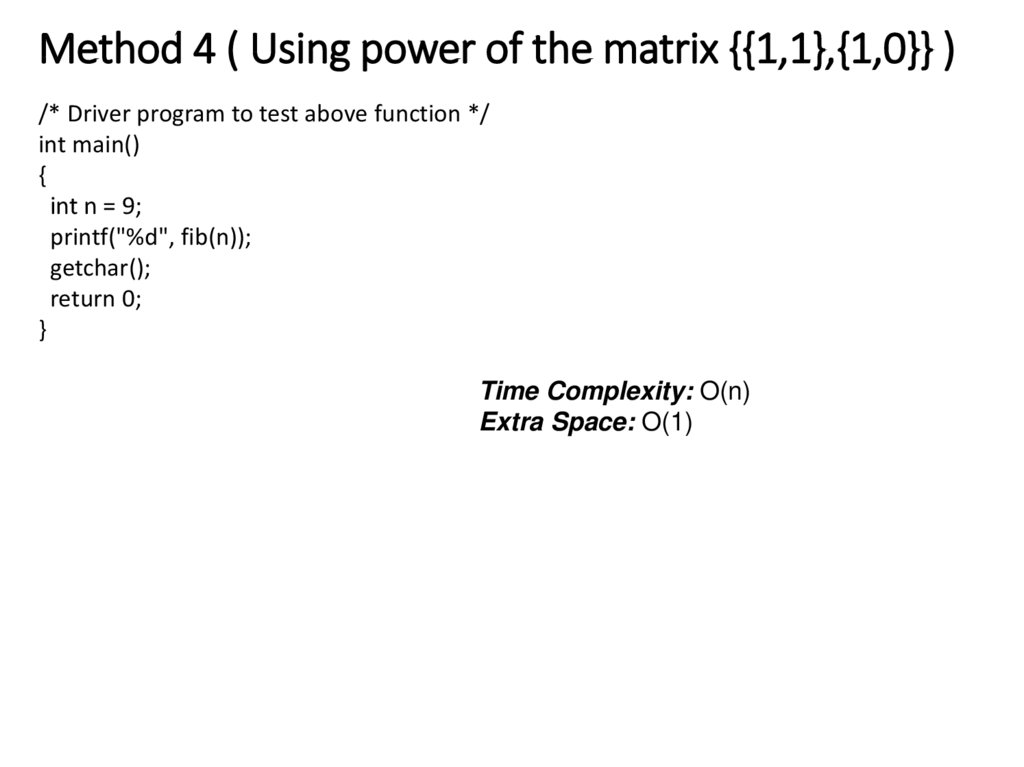
/* Driver program to test above function */
int main()
{
int n = 9;
printf("%d", fib(n));
getchar();
return 0;
}
Time Complexity: O(n)
Extra Space: O(1)

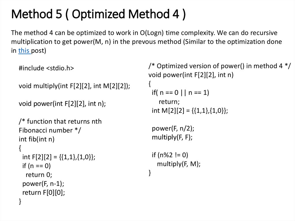
25. Method 5 ( Optimized Method 4 )

The method 4 can be optimized to work in O(Logn) time complexity. We can do recursive
multiplication to get power(M, n) in the prevous method (Similar to the optimization done
in this post)
#include <stdio.h>
void multiply(int F[2][2], int M[2][2]);
void power(int F[2][2], int n);
/* function that returns nth
Fibonacci number */
int fib(int n)
{
int F[2][2] = {{1,1},{1,0}};
if (n == 0)
return 0;
power(F, n-1);
return F[0][0];
}
/* Optimized version of power() in method 4 */
void power(int F[2][2], int n)
{
if( n == 0 || n == 1)
return;
int M[2][2] = {{1,1},{1,0}};
power(F, n/2);
multiply(F, F);
if (n%2 != 0)
multiply(F, M);
}

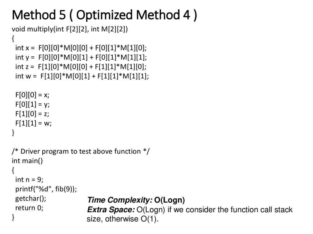
26. Method 5 ( Optimized Method 4 )

void multiply(int F[2][2], int M[2][2])
{
int x = F[0][0]*M[0][0] + F[0][1]*M[1][0];
int y = F[0][0]*M[0][1] + F[0][1]*M[1][1];
int z = F[1][0]*M[0][0] + F[1][1]*M[1][0];
int w = F[1][0]*M[0][1] + F[1][1]*M[1][1];
F[0][0] = x;
F[0][1] = y;
F[1][0] = z;
F[1][1] = w;
}
/* Driver program to test above function */
int main()
{
int n = 9;
printf("%d", fib(9));
getchar();
Time Complexity: O(Logn)
return 0;
Extra Space: O(Logn) if we consider the function call stack
}
size, otherwise O(1).

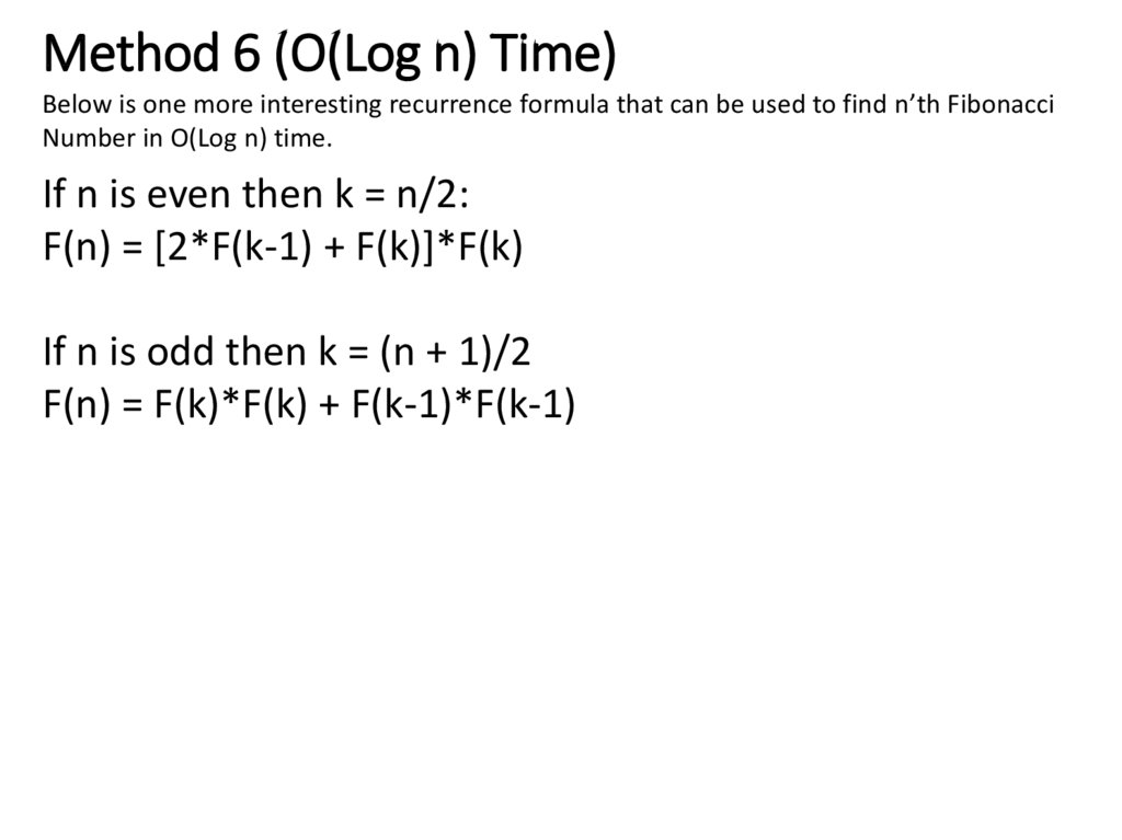
27. Method 6 (O(Log n) Time)

Below is one more interesting recurrence formula that can be used to find n’th Fibonacci
Number in O(Log n) time.
If n is even then k = n/2:
F(n) = [2*F(k-1) + F(k)]*F(k)
If n is odd then k = (n + 1)/2
F(n) = F(k)*F(k) + F(k-1)*F(k-1)

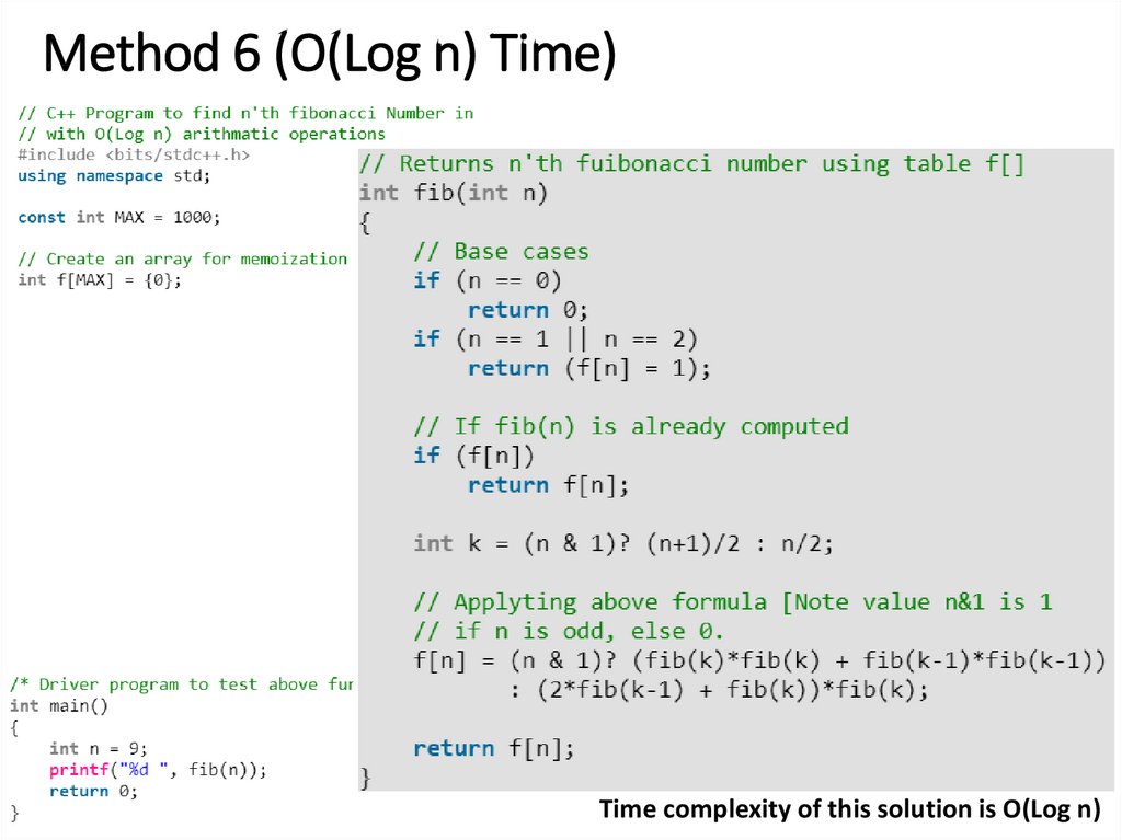
28. Method 6 (O(Log n) Time)

Time complexity of this solution is O(Log n)

29. Method 7 Another approach:(Using formula)

In this method we directly implement the formula for nth term in the fibonacci series.
Fn = {[(√5 + 1)/2] ^ n} / √5
Reference:
http://www.maths.surrey.ac.uk/hosted-sites/R.Knott/Fibonacci/fibFormula.html
Time Complexity: O(1)
Space Complexity: O(1)

30. 5 BDD & ROBDD

5 BDD & ROBDD
In computer science, a binary decision diagram (BDD) or branching program is a data
structure that is used to represent a Boolean function. On a more abstract level, BDDs can
be considered as a compressed representation of sets or relations. Unlike other
compressed representations, operations are performed directly on the compressed
representation, i.e. without decompression. Other data structures used to
represent Boolean functions include negation normal form (NNF), Zhegalkin polynomials,
and propositional directed acyclic graphs (PDAG).
In popular usage, the term BDD almost always refers to Reduced Ordered Binary
Decision Diagram (ROBDD in the literature, used when the ordering and reduction
aspects need to be emphasized). The advantage of an ROBDD is that it is
canonical (unique) for a particular function and variable order.[1] This property
makes it useful in functional equivalence checking and other operations like
functional technology mapping.
A path from the root node to the 1-terminal represents a (possibly partial) variable
assignment for which the represented Boolean function is true. As the path
descends to a low (or high) child from a node, then that node's variable is assigned
to 0 (respectively 1).
https://en.wikipedia.org/wiki/Binary_decision_diagram

31. 5 Implementing ROBDDs

In the implementation of ROBDDs, dynamic programming plays
a pervasive role. Binary decision diagrams (BDDs) satisfying two
conditions:
• Irredundancy: The low and high successors of every node are
distinct.
• Uniqueness: There are no two distinct nodes testing the same
variable with the same successors.
These two conditions guarantee canonicity of the
representation of boolean functions and also make the
data structure efficient in many common cases.

32. 6 Encoding the n-Queens Problem

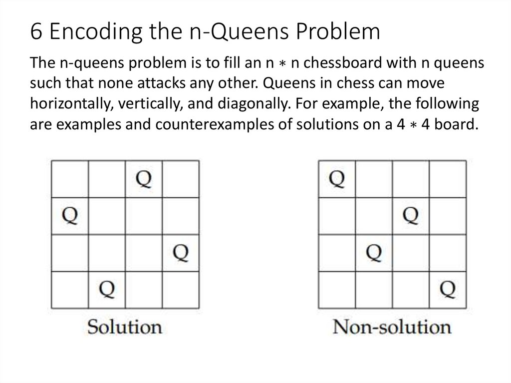
The n-queens problem is to fill an n ∗ n chessboard with n queens
such that none attacks any other. Queens in chess can move
horizontally, vertically, and diagonally. For example, the following
are examples and counterexamples of solutions on a 4 ∗ 4 board.

33. 6 Encoding the n-Queens Problem

We would like to encode n-queens problems as ROBDDS. The idea
is to assign a boolean variable to each square, where a value of 1
means that the square is occupied by a queen, and a 0 means that
the square is empty. We write these variables as xij for the square
at column i and row j.
Now we need to generate constraints on these boolean variables
such that a correct solution will be evaluated as true (1) and an
incorrect situation will be evaluated as false (0).

34. 6 Encoding the n-Queens Problem

For example, to encode that the column 0 has at least one queen
on a 4 ∗ 4 board, we would write
x00 ∨ x01 ∨ x02 ∨ x03
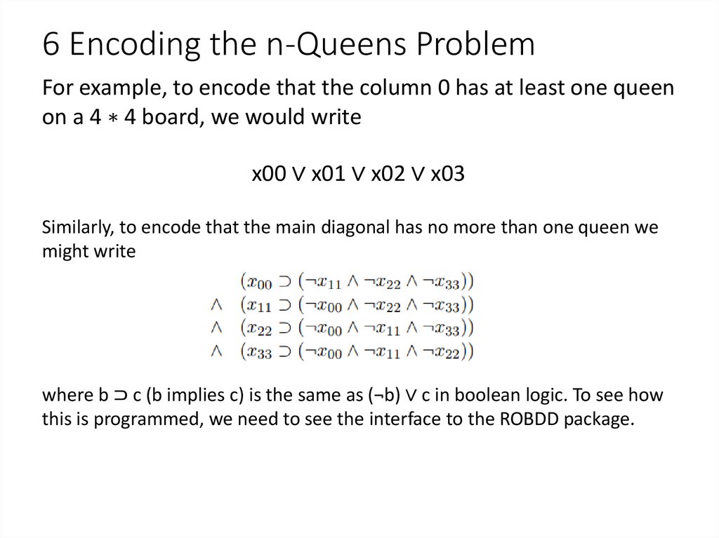
Similarly, to encode that the main diagonal has no more than one queen we
might write
where b ⊃ c (b implies c) is the same as (¬b) ∨ c in boolean logic. To see how
this is programmed, we need to see the interface to the ROBDD package.

35. 6 Encoding the n-Queens Problem

typedef struct bdd* bdd;
typedef int bdd_node;
bdd bdd_new(int k); /* k variables */
void bdd_free(bdd B);
int bdd_size(bdd B); /* total number of nodes */
bdd_node make(bdd B, int var, bdd_node low,
bdd_node high);
bdd_node apply(bdd B, int (*func)(int b1, int
b2), bdd_node u1, bdd_node u2);
int satcount(bdd B, bdd_node u);
void onesat(bdd B, bdd_node u);
void allsat(bdd B, bdd_node u);

36. 6 Encoding the n-Queens Problem

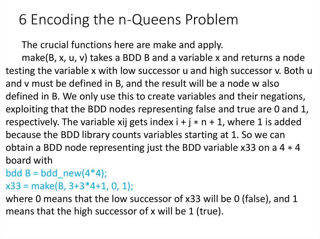
The crucial functions here are make and apply.
make(B, x, u, v) takes a BDD B and a variable x and returns a node
testing the variable x with low successor u and high successor v. Both u
and v must be defined in B, and the result will be a node w also
defined in B. We only use this to create variables and their negations,
exploiting that the BDD nodes representing false and true are 0 and 1,
respectively. The variable xij gets index i + j ∗ n + 1, where 1 is added
because the BDD library counts variables starting at 1. So we can
obtain a BDD node representing just the BDD variable x33 on a 4 ∗ 4
board with
bdd B = bdd_new(4*4);
x33 = make(B, 3+3*4+1, 0, 1);
where 0 means that the low successor of x33 will be 0 (false), and 1
means that the high successor of x will be 1 (true).

37. 6 Encoding the n-Queens Problem

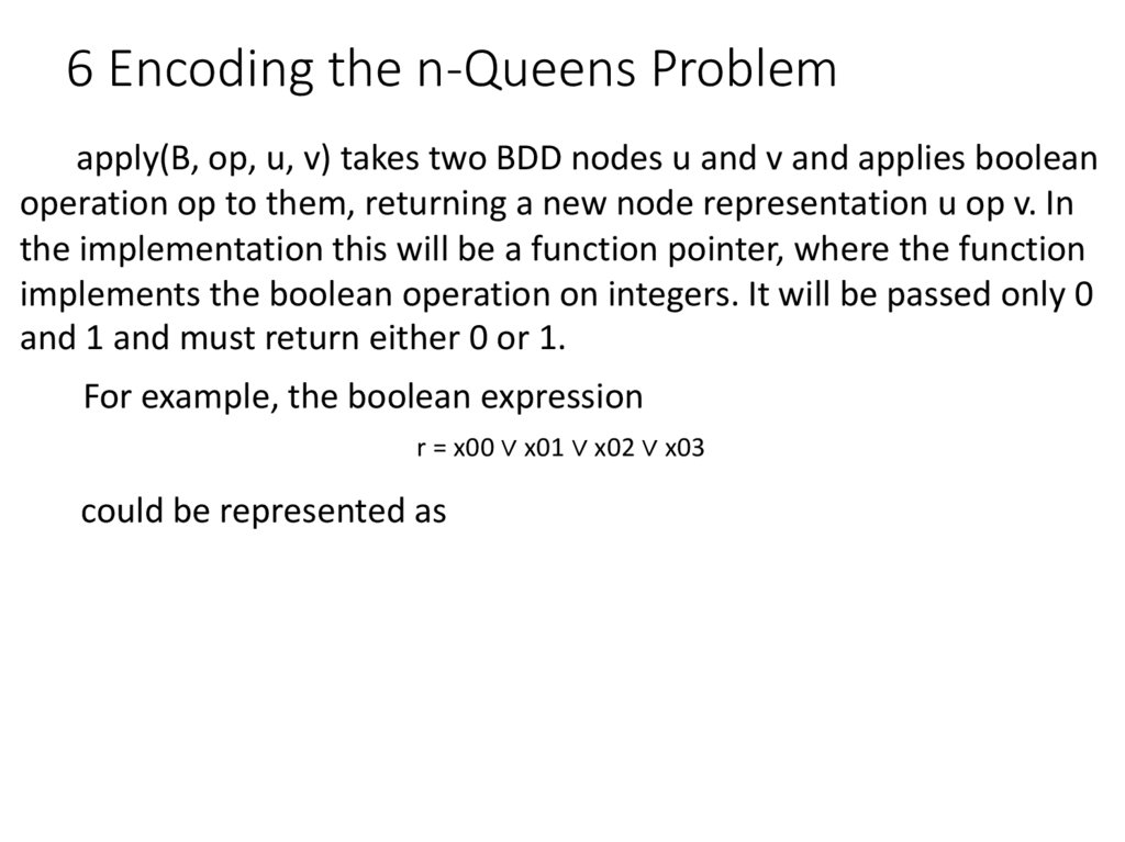
apply(B, op, u, v) takes two BDD nodes u and v and applies boolean
operation op to them, returning a new node representation u op v. In
the implementation this will be a function pointer, where the function
implements the boolean operation on integers. It will be passed only 0
and 1 and must return either 0 or 1.
For example, the boolean expression
r = x00 ∨ x01 ∨ x02 ∨ x03
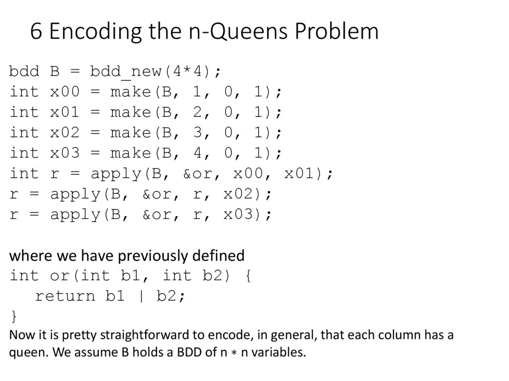
could be represented as

38. 6 Encoding the n-Queens Problem

bdd
int
int
int
int
int
r =
r =
B = bdd_new(4*4);
x00 = make(B, 1, 0, 1);
x01 = make(B, 2, 0, 1);
x02 = make(B, 3, 0, 1);
x03 = make(B, 4, 0, 1);
r = apply(B, &or, x00, x01);
apply(B, &or, r, x02);
apply(B, &or, r, x03);
where we have previously defined
int or(int b1, int b2) {
return b1 | b2;
}
Now it is pretty straightforward to encode, in general, that each column has a
queen. We assume B holds a BDD of n ∗ n variables.

39. 6 Encoding the n-Queens Problem

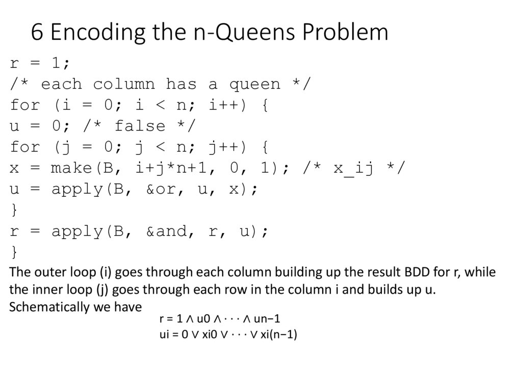
r = 1;
/* each column has a queen */
for (i = 0; i < n; i++) {
u = 0; /* false */
for (j = 0; j < n; j++) {
x = make(B, i+j*n+1, 0, 1); /* x_ij */
u = apply(B, &or, u, x);
}
r = apply(B, &and, r, u);
}
The outer loop (i) goes through each column building up the result BDD for r, while
the inner loop (j) goes through each row in the column i and builds up u.
Schematically we have
r = 1 ∧ u0 ∧ · · · ∧ un−1
ui = 0 ∨ xi0 ∨ · · · ∨ xi(n−1)