3.22M

Категория:

Программирование

Dynamic Programming

Dynamic Programming
• Dynamic programming is a very powerful,
general tool for solving optimization problems.
• Once understood it is relatively easy to apply,
but many people have trouble understanding
it.

5.

Greedy Algorithms
• Greedy algorithms focus on making the best
local choice at each decision point.
• For example, a natural way to compute a
shortest path from x to y might be to walk out
of x, repeatedly following the cheapest edge
until we get to y. WRONG!
• In the absence of a correctness proof greedy
algorithms are very likely to fail.

6.

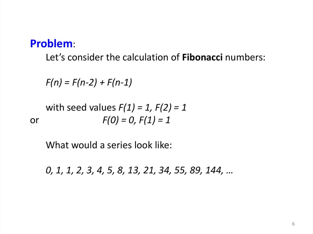
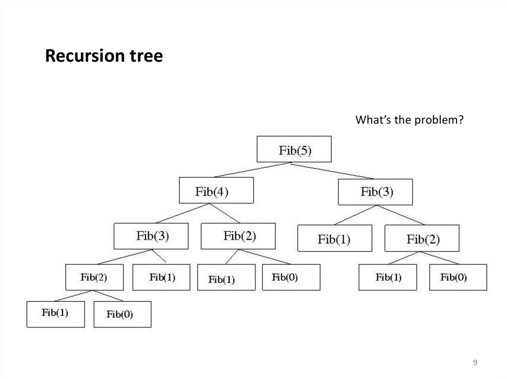
Problem:
Let’s consider the calculation of Fibonacci numbers:
F(n) = F(n-2) + F(n-1)
with seed values F(1) = 1, F(2) = 1
or
F(0) = 0, F(1) = 1
What would a series look like:
0, 1, 1, 2, 3, 4, 5, 8, 13, 21, 34, 55, 89, 144, …
6

7.

Recursive Algorithm:
Fib(n)
{
if (n == 0)
return 0;
if (n == 1)
return 1;
Return Fib(n-1)+Fib(n-2)
}
7

8.

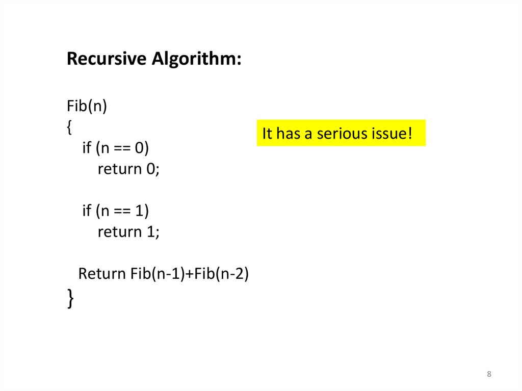
Recursive Algorithm:
Fib(n)
{
if (n == 0)
return 0;
It has a serious issue!
if (n == 1)
return 1;
Return Fib(n-1)+Fib(n-2)
}
8

9.

Recursion tree
What’s the problem?
9

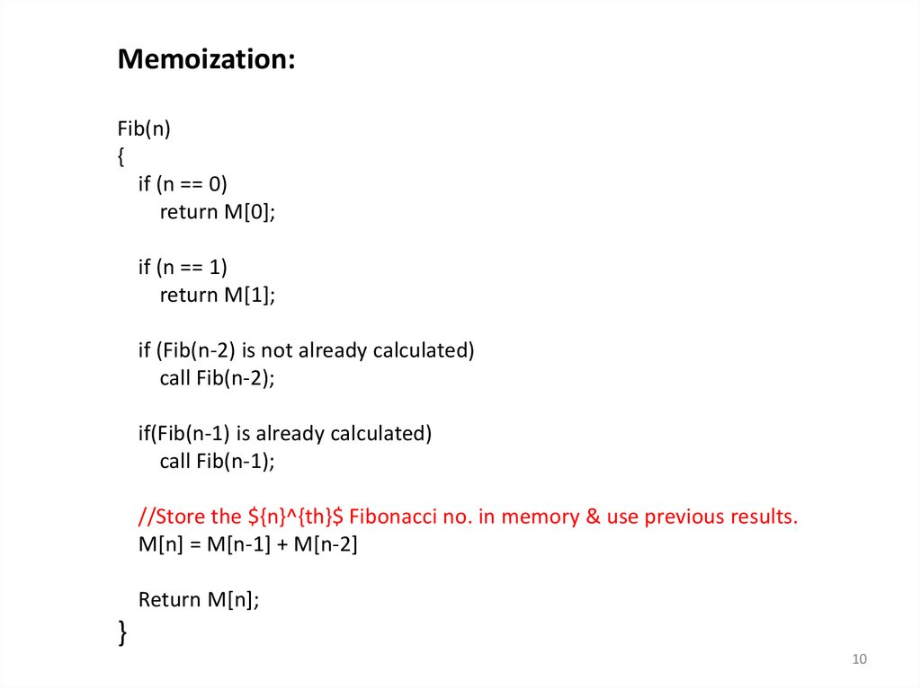
10.

Memoization:
Fib(n)
{
if (n == 0)
return M[0];
if (n == 1)
return M[1];
if (Fib(n-2) is not already calculated)
call Fib(n-2);
if(Fib(n-1) is already calculated)
call Fib(n-1);
//Store the ${n}^{th}$ Fibonacci no. in memory & use previous results.
M[n] = M[n-1] + M[n-2]
Return M[n];
}
10

11.

already calculated …
11

12.

Dynamic programming
- Main approach: recursive, holds answers to a sub problem in a
table, can be used without recomputing.
- Can be formulated both via recursion and saving results in a
table (memoization). Typically, we first formulate the recursive
solution and then turn it into recursion plus dynamic
programming via memoization or bottom-up.
-”programming” as in tabular not programming code
12

13.

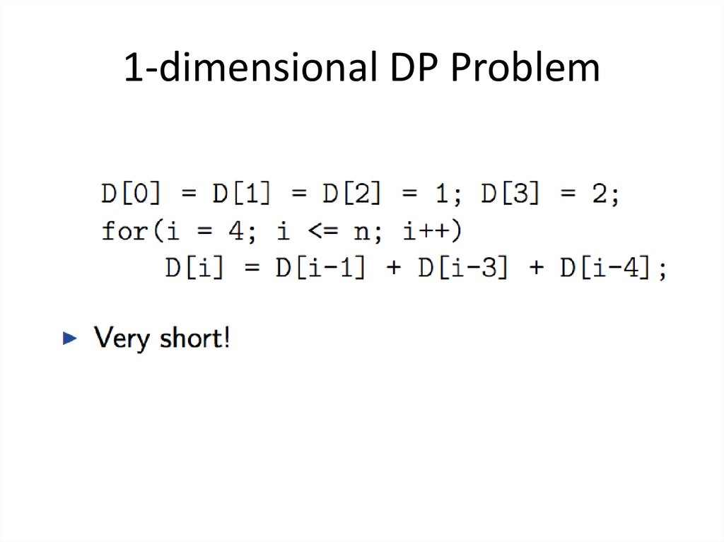
1-dimensional DP Problem

14.

1-dimensional DP Problem

15.

1-dimensional DP Problem

16.

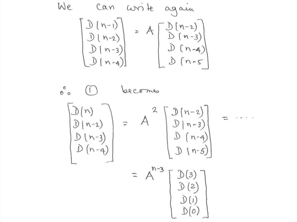
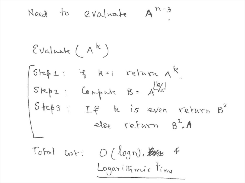
1-dimensional DP Problem

17.

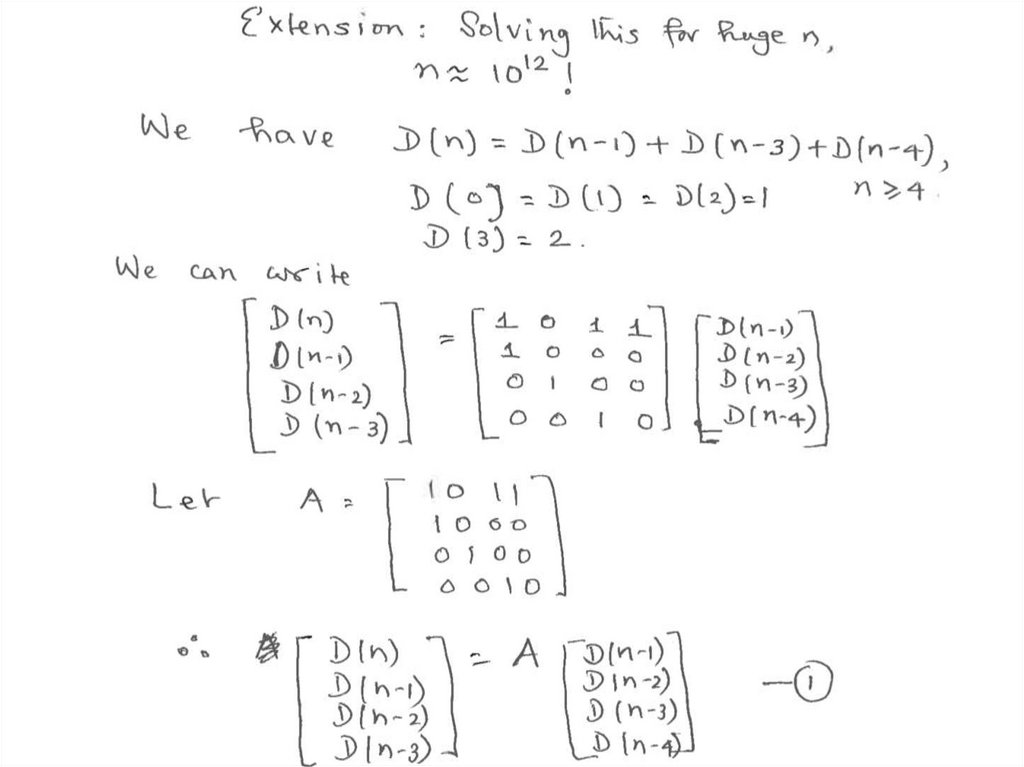
What happens when n is extremely
large?

18.

19.

20.

21.

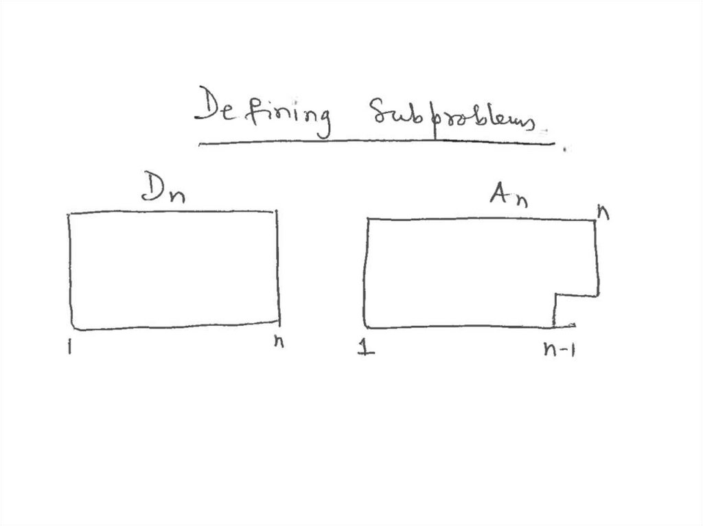
Tri Tiling

22.

Tri Tiling

23.

Tri Tiling

24.

25.

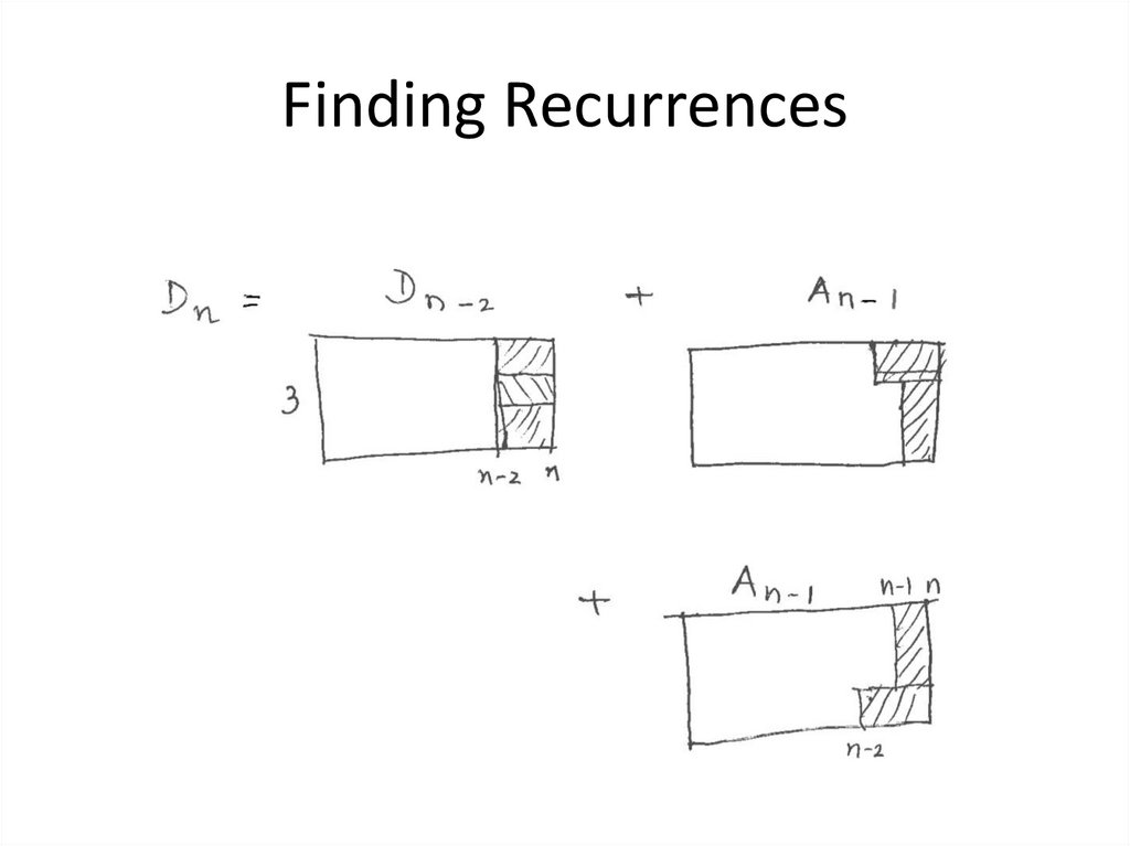
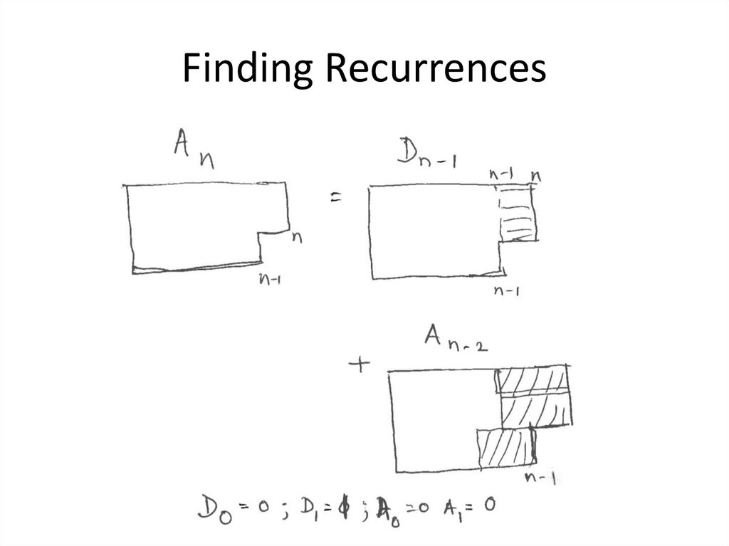
Finding Recurrences

26.

Finding Recurrences

27.

Extension
• Solving the problem for n x m grids, where n is
small, say n ≤ 10.
– How many subproblems do we consider?

28.

29.

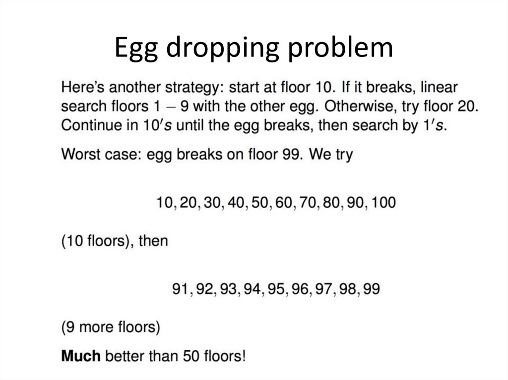
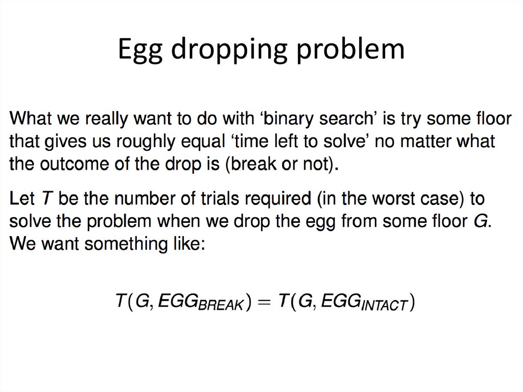
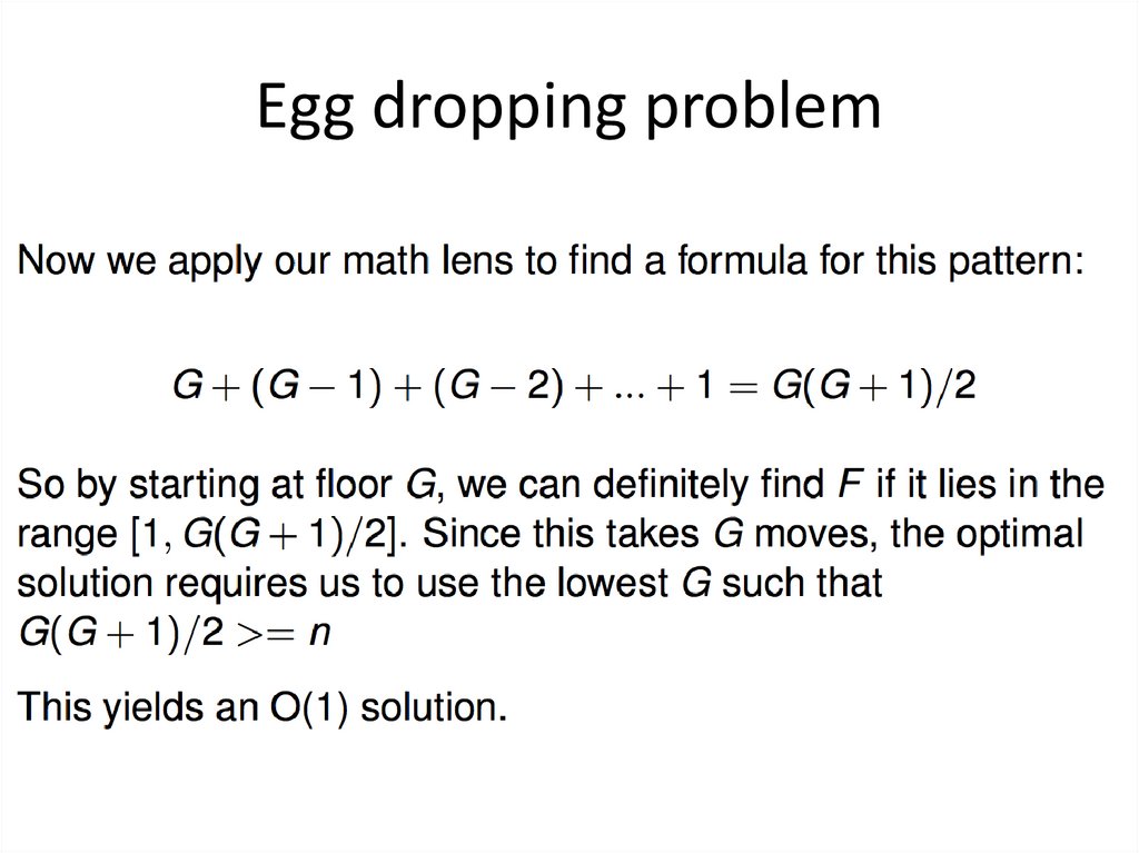
Egg dropping problem

30.

Egg dropping problem

31.

Egg dropping problem

32.

Egg dropping problem

33.

Egg dropping problem

34.

Egg dropping problem

35.

Egg dropping problem

36.

Egg dropping problem(n eggs)
Dynamic Programming Approach
D[j,m] : There are j floors and m eggs. Like to find the
floors with the largest value from which an egg, when
dropped doesn’t crack.
Here the egg cracked
when dropped from
floor g.

37.

Egg dropping problem(n eggs)
Dynamic Programming Approach
DP[j,m] : There are j floors and m eggs. Like to find the
floors with the largest value from which an egg, when
dropped doesn’t crack.
Here the egg didn’t
crack when dropped
from floor g.
Here the egg cracked
when dropped from
floor g.

38.

39.

40.

41.

42.

43.

44.

45.

46.

47.

48.

Coin-change Problem
• To find the minimum number of Canadian coins
to make any amount, the greedy method always
works.
– At each step select the largest denomination not
going over the desired amount.

49.

Coin-change Problem
• The greedy method doesn’t work if we didn’t
have 5¢ coin.
– For 31¢, the greedy solution is 25 +1+1+1+1+1+1
– But we can do it with 10+10+10+1
• The greedy method also wouldn’t work if we had
a 21¢ coin
– For 63¢, the greedy solution is 25+25+10+1+1+1
– But we can do it with 21+21+21

50.

Coin set for examples
• For the following examples, we will assume
coins in the following denominations:
1¢ 5¢ 10¢ 21¢ 25¢
• We’ll use 63¢ as our goal

51.

A solution
• We can reduce the problem recursively by choosing the
first coin, and solving for the amount that is left
• For 63¢:
– One 1¢ coin plus the best solution for 62¢
– One 5¢ coin plus the best solution for 58¢
– One 10¢ coin plus the best solution for 53¢
– One 21¢ coin plus the best solution for 42¢
– One 25¢ coin plus the best solution for 38¢
• Choose the best solution from among the 5 given above
• We solve 5 recursive problems.
• This is a very expensive algorithm

52.

A dynamic programming
solution
• Idea: Solve first for one cent, then two cents,
then three cents, etc., up to the desired amount
– Save each answer in an array !
• For each new amount N, combine a selected
pairs of previous answers which sum to N
– For example, to find the solution for 13¢,
• First, solve for all of 1¢, 2¢, 3¢, ..., 12¢
• Next, choose the best solution among:
– Solution for 1¢ + solution for 12¢
– Solution for 5¢ + solution for 8¢
– Solution for 10¢ + solution for 3¢

53.

A dynamic programming
solution
• Let T(n) be the number of coins taken to
dispense n¢.
• The recurrence relation
– T(n) = min {T(n-1), T(n-5), T(n-10), T(n-25)} + 1, n ≥ 26
– T(c) is known for n ≤ 25
• It is exponential if we are not careful.
• The bottom-up approach is the best.
• Memoization idea also can be used.

54.

A dynamic programming
solution
• The dynamic programming algorithm is O(N*K)
where N is the desired amount and K is the
number of different kind of coins.

55.

Comparison with divide-and-conquer
• Divide-and-conquer algorithms split a problem
into separate subproblems, solve the subproblems,
and combine the results for a solution to the
original problem
– Example: Quicksort
– Example: Mergesort
– Example: Binary search
• Divide-and-conquer algorithms can be
thought of as top-down algorithms

56.

Comparison with divide-and-conquer
• In contrast, a dynamic programming algorithm
proceeds by solving small problems, remembering
the results, then combining them to find the solution
to larger problems
• Dynamic programming can be thought of as bottomup

57.

The principle of optimality, I
• Dynamic programming is a technique for
finding an optimal solution
• The principle of optimality applies if the
optimal solution to a problem can be obtained
by combining the optimal solutions to all
subproblems.

58.

The principle of optimality, I
• Example: Consider the problem of making N¢
with the fewest number of coins
– Either there is an N¢ coin, or
– The set of coins making up an optimal solution for
N¢ can be divided into two nonempty subsets, n1¢
and n2¢
• If either subset, n1¢ or n2¢, can be made with fewer
coins, then clearly N¢ can be made with fewer coins,
hence solution was not optimal

59.

The principle of optimality, II
• The principle of optimality holds if
– Every optimal solution to a problem contains...
– ...optimal solutions to all subproblems
• The principle of optimality does not say
– If you have optimal solutions to all subproblems...
– ...then you can combine them to get an optimal
solution

60.

The principle of optimality, II
• Example: In coin problem,
– The optimal solution to 7¢ is 5¢ + 1¢ + 1¢, and
– The optimal solution to 6¢ is 5¢ + 1¢, but
– The optimal solution to 13¢ is not 5¢ + 1¢ + 1¢ + 5¢
+ 1¢
• But there is some way of dividing up 13¢ into
subsets with optimal solutions that will give an
optimal solution for 13¢
– Hence, the principle of optimality holds for this
problem

61.

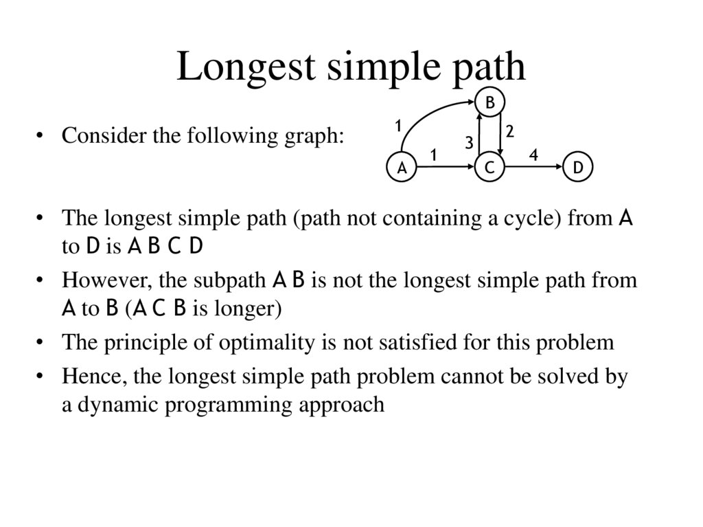
Longest simple path
B
• Consider the following graph:
1
A
1
2
3
C
4
D
• The longest simple path (path not containing a cycle) from A
to D is A B C D
• However, the subpath A B is not the longest simple path from
A to B (A C B is longer)
• The principle of optimality is not satisfied for this problem
• Hence, the longest simple path problem cannot be solved by
a dynamic programming approach

62.

• Example: In coin problem,
– The optimal solution to 7¢ is 5¢ + 1¢ + 1¢, and
– The optimal solution to 6¢ is 5¢ + 1¢, but
– The optimal solution to 13¢ is not 5¢ + 1¢ + 1¢ + 5¢
+ 1¢
• But there is some way of dividing up 13¢ into
subsets with optimal solutions that will give an
optimal solution for 13¢
– Hence, the principle of optimality holds for this
problem

63.

The 0-1 knapsack problem
• A thief breaks into a house, carrying a
knapsack...
– He can carry up to 25 pounds of loot
– He has to choose which of N items to steal
• Each item has some weight and some value
• “0-1” because each item is stolen (1) or not stolen (0)
– He has to select the items to steal in order to
maximize the value of his loot, but cannot exceed 25
pounds

64.

The 0-1 knapsack problem
• A greedy algorithm does not find an optimal
solution
• A dynamic programming algorithm works well.

65.

The 0-1 knapsack problem
• This is similar to, but not identical to, the coins
problem
– In the coins problem, we had to make an exact
amount of change
– In the 0-1 knapsack problem, we can’t exceed the
weight limit, but the optimal solution may be less
than the weight limit
– The dynamic programming solution is similar to that
of the coins problem

66.

Steps for Solving DP Problems
• Define subproblems
• Write down the recurrence that relates
subproblems
• Recognize and solve the base cases
• Each step is very important.

67.

Comments
• Dynamic programming relies on working
“from the bottom up” and saving the results of
solving simpler problems
– These solutions to simpler problems are then used
to compute the solution to more complex problems
• Dynamic programming solutions can often be
quite complex and tricky

68.

Comments
• Dynamic programming is used for optimization
problems, especially ones that would otherwise
take exponential time
– Only problems that satisfy the principle of optimality
are suitable for dynamic programming solutions
• Since exponential time is unacceptable for all but
the smallest problems, dynamic programming is
sometimes essential.

English Русский Правила