05 II. Inflation. Its causes, effects, and social costs

1.

Dr.
S.Sh.Sagandyko
va
Prepared by:
MACROECONOMICS
LECTURE
5
___
INFLATION:
ITS CAUSES, EFFECTS, AND SOCIAL COSTS
1

2.

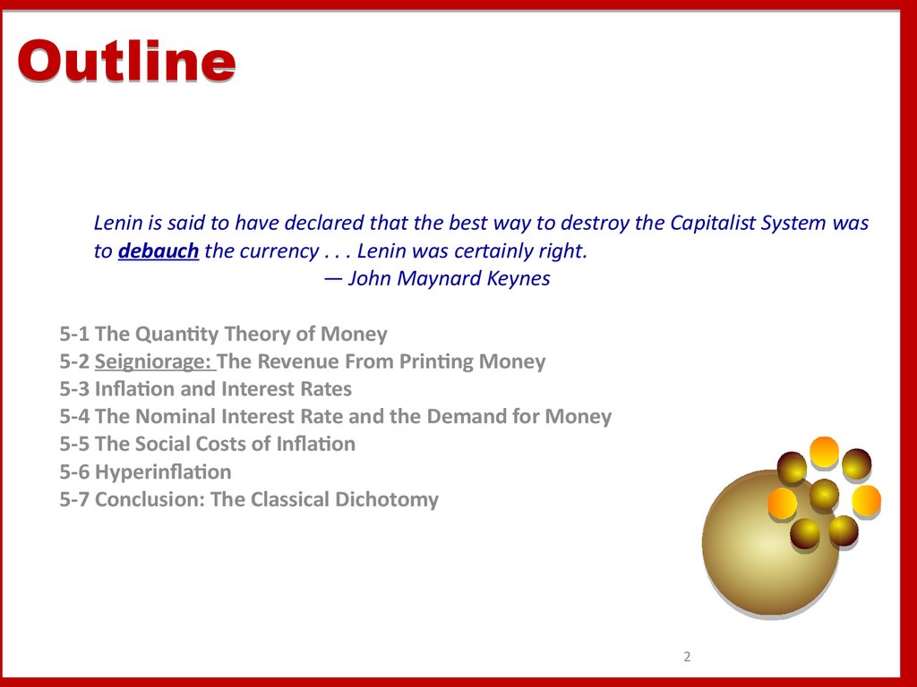
Outline
Lenin is said to have declared that the best way to destroy the Capitalist System was
to debauch the currency . . . Lenin was certainly right.
— John Maynard Keynes
5-1 The Quantity Theory of Money
5-2 Seigniorage: The Revenue From Printing Money
5-3 Inflation and Interest Rates
5-4 The Nominal Interest Rate and the Demand for Money
5-5 The Social Costs of Inflation
5-6 Hyperinflation
5-7 Conclusion: The Classical Dichotomy
2

3. 5-1 The Quantity Theory of Money

Оverall increase in prices is called inflation.
The rate of inflation - the percentage change in the overall level of
prices - varies greatly over time and across countries.
Hyperinflation:
A classic example is Germany in 1923, when
prices increased an average of 500 percent per month.
Introduction
The revenue that governments can raise by printing money, called
the inflation tax.
Money is the stock of assets that can be readily used to make
transactions.
• Roughly speaking, the $s in the hands of the public make up the
nation’s stock of money.
3

4. 5-1 The Quantity Theory of Money

Transactions and the Quantity Equation
From Transactions to Income
The Money Demand Function and the Quantity Equation
The Assumption of Constant Velocity
Money, Prices, and Infation
5-1 The Quantity Theory of Money
Money * Velocity = Price * Transactions
M * V = P * T.
T is the number of times in a year that G&S services are exchanged
for money.
P is the number of $s exchanged.
PT is the number of $s exchanged in a year.
MV - the money used to make the transactions.
M is the quantity of money.
V, called the transactions velocity of money, measures the rate at
which money circulates in the economy.
• The number of times a $ bill changes hands in a given period of
time.
4

5. 5-1 The Quantity Theory of Money

Transactions and the Quantity Equation
From Transactions to Income
The Money Demand Function and the Quantity Equation
The Assumption of Constant Velocity
Money, Prices, and Infation
5-1 The Quantity Theory of Money
For example,
T = 60 loaves per year, and P = $0.50 per loaf.
• The total number of $ s exchanged is
PT = $0.50/loaf * 60 loaves/year = $30/year.
the quantity of Money in the economy is $10.
• V = PT/M = ($30/year)/($10) = 3 times per year.
5

6. 5-1 The Quantity Theory of Money

Money * Velocity = Price * Output
M * V = P * Y.
Transactions and the Quantity Equation
From Transactions to Income
The Money Demand Function and the Quantity Equation
The Assumption of Constant Velocity
Money, Prices, and Infation
Y is real GDP;
P, the GDP deflator;
PY, nominal GDP.
Because Y is also total income,
V in this version of the quantity equation is called
the income velocity of money.
It tells us
the number of times
a $ bill
enters someone’s income
in a given period of time.
This version of the quantity equation is the most common.
6

7. 5-1 The Quantity Theory of Money

Transactions and the Quantity Equation
From Transactions to Income
The Money Demand Function and the Quantity Equation
The Assumption of Constant Velocity
Money, Prices, and Infation
5-1 The Quantity Theory of Money
M/P, is called real money balances.
M * V = P * Y.
For example,
• economy that produces only bread.
• If the M is $10, the P of a loaf is $0.50, then
• real money balances are 20 loaves of bread
A money demand function is an equation that shows the
determinants of the quantity of real money balances people wish to
hold.
= kY,
• k is a constant that tells us
• how much money people want to hold for every dollar of income
DEMAND for (M/P)d must equal the SUPPLY M/P.
→
M/P = kY
→ M(1/k) = PY
→
When people want to hold
• a lot of M (k is large), (V is small).
• a little M (k is small), (V is large).
MV = PY, where V = 1/k.
7

8. 5-1 The Quantity Theory of Money

Transactions and the Quantity Equation
From Transactions to Income
The Money Demand Function and the Quantity Equation
The Assumption of Constant Velocity
Money, Prices, and Infation
5-1 The Quantity Theory of Money
Yet if we make the additional assumption
that the velocity of money is constant,
then the quantity equation becomes a useful theory
about the effects of money, called the
quantity theory of money.
The quantity equation can be seen as a theory of what determines
nominal GDP.
M = P Y,
=> change in the quantity of money (M) must cause a proportionate
change in nominal GDP (PY).
That is, if velocity is fixed, the quantity of money determines the
dollar value of the economy’s output.
8

9. 5-1 The Quantity Theory of Money

Transactions and the Quantity Equation
From Transactions to Income
The Money Demand Function and the Quantity Equation
The Assumption of Constant Velocity
Money, Prices, and Inflation
% Change in M + % Change in V = % Change in P + % Change in Y.
1. % Change in M is under the control of the CB.
2. % Change in V reflects shifts in M demand; V is constant, so %
Change in V = 0.
3. % Change in P is the rate of inflation; this is the variable that we
would like to explain.
4. % Change in Y ~on growth in the factors of production and on
technological progress.
1. This analysis tells us that the growth in the M supply
determines the rate of inflation.
.Thus, the quantity theory of money states that the CB, which
controls the M supply, has ultimate control over the rate of inflation.
•. If the CB keeps the M supply stable, the price level will be stable.
•. If the CB increases the M supply rapidly, the price level will rise
rapidly.
9

10. Inflation and Money Growth

Case
Study
Inflation and Money Growth

11. Inflation and Money Growth

Case
Study
Inflation and Money Growth

12. 5-2 Seigniorage: The Revenue From Printing Money

1. The revenue raised by the printing of money is called SEIGNIORAGE.
2. Today this right belongs to the central government, and it is one source
of revenue.
3. When the government prints money to finance expenditure, it
increases the money supply.
4. The increase in the money supply, in turn, causes inflation.
5. Printing money to raise revenue is like imposing an inflation tax.
a. when the government prints new money for its use,
it makes the old money in the hands of the public less valuable.
6. In the United States, the amount has been small: seigniorage has
usually accounted for less than 3 % of government revenue.
12

13. Paying for the American Revolution

Although seigniorage has not been a major source of revenue for the U.S.
Government in recent history, the situation was very different two centuries
ago.
Beginning in 1775, the Continental Congress needed to find a way to finance the
Revolution, but it had limited ability to raise revenue through taxation.
It therefore relied on the printing of fiat money to help pay for the war.
When the new nation won its independence, there was a natural skepticism
Case
Study
about fiat money.
Congress passed the Mint Act of 1792, which established gold and silver as the
basis for a new system of commodity money.

14. 5-3 Inflation and Interest Rates

Two Interest Rates: Real and Nominal
The Fisher Efect
Two Real Interest Rates: Ex Ante and Ex Post
5-3 Inflation and Interest Rates
The interest rate that the bank pays is called the nominal interest
rate,
and the increase in your purchasing power is called the real interest
rate.
If
i denotes the nominal interest rate,
r the real interest rate, and
π the rate of inflation,
then the relationship among these three variables can be written as
r=i–π.
14

15. 5-3 Inflation and Interest Rates

Two Interest Rates: Real and Nominal
The Fisher Effect
Two Real Interest Rates: Ex Ante and Ex Post
5-3 Inflation and Interest Rates
Rearranging terms in our equation for the r , we can show that
the i is the sum of the r and the infation rate π :
i=r+π.
The equation written in this way is called the Fisher equation, after
economist Irving Fisher (1867–1947).
1. According to the quantity theory,
• an increase in the rate of money growth of 1 percent causes
• a 1 percent increase in the rate of inflation.
2. According to the Fisher equation,
• a 1 percent increase in the rate of inflation in turn causes
• a 1 percent increase in the nominal interest rate.
.The one-for-one relation between the inflation rate and the
nominal interest rate is called the Fisher effect.
1% ↑ => 1% i ↑
15

16. Inflation and Nominal Interest Rates

Case
Study
Inflation and Nominal Interest Rates

17. Inflation and Nominal Interest Rates

Case
Study
Inflation and Nominal Interest Rates

18. 5-3 Inflation and Interest Rates

Two Interest Rates: Real and Nominal
The Fisher Effect
Two Real Interest Rates: Ex Ante and Ex Post
5-3 Inflation and Interest Rates
1. The r that the borrower and lender expect when the loan is made,
called the ex ante r ,
2. the r that is actually realized, called the ex post r .
Let denote actual future inflation π and Eπ the expectation of future
inflation.
The ex ante r is i – Eπ,
the ex post r is i –π .
How does this distinction between actual and expected
inflation modify the Fisher effect?
The i cannot adjust to actual infation, because
actual inflation is not known when the i is set.
The i can adjust only to expected inflation.
The Fisher effect is more precisely written as i = r + Eπ :
•. The ex ante r is determined by equilibrium in the market for G&S.
•. The i moves one-for-one with changes in expected infation E.
18

19. Nominal Interest Rates in the Nineteenth Century

Although recent data show a positive relationship between nominal interest
rates and inflation rates, this finding is not universal.
In data from the late nineteenth and early twentieth centuries, high nominal
interest rates did not accompany high inflation.
Case
Study
The apparent absence of any Fisher effect during this time puzzled Irving Fisher.
• He suggested that inflation “caught merchants napping.’’

20. 5-4 The Nominal Interest Rate and the Demand for Money

The money you hold in your wallet does not earn interest.
If you deposited it in a savings account, you would earn the nominal
interest rate.
The Cost of Holding Money
Future Money and Current Prices
Therefore, the nominal interest rate is the opportunity cost of
holding money.
You will or you will not.
The letter L is used to denote money demand because money is the
economy’s most Liquid asset.
This equation states that the demand for the liquidity of real money
balances is a function of income and the nominal interest rate.
1. The higher the level of income Y, the greater the demand for real
money balances.
2. The higher the nominal interest rate i, the lower the demand for
real money balances.

21. 5-4 The Nominal Interest Rate and the Demand for Money

The Cost of Holding Money
Future Money and Current Prices
5-4 The Nominal Interest Rate and the Demand for Money

22. 5-4 The Nominal Interest Rate and the Demand for Money

The Cost of Holding Money
Future Money and Current Prices
5-4 The Nominal Interest Rate and the Demand for Money
• Consider how the introduction of this last link afects our theory
of the price level.
• First, equate the supply of real money balances M/P to the
demand L(i, Y):
1. M/P = L(i, Y).
• Next, use the Fisher equation to write the nominal interest rate
as the sum of the real interest rate and expected infation:
2. M/P = L(r + Eπ, Y).
• This equation states that the level of real money balances
depends on the expected rate of infation.
.P ~ M , if i and Y constant
.If i = r+ Eπ, Eπ ~ on M
.Expectations of higher money growth in the future lead to a
higher price level today.

23. 5-5 The Social Costs of Inflation

The Layman’s View and the Classical Response
The Costs of Expected Infation
The Costs of Unexpected Infation
One Benefit of Infation
5-5 The Social Costs of Inflation
If you ask the average person why inflation is a social problem, he
will probably answer that inflation makes him poorer.
“Each year my boss gives me a raise, but prices go up and that takes
some of my raise away from me.’’
The implicit assumption in this statement is that if there were no
inflation, he would get the same raise and be able to buy more
goods.
To the surprise of many laymen,
some economists argue that the costs of inflation are small.

24. What Economists and the Public Say About Inflation

As we have been discussing, laymen and economists hold very diferent views
about the costs of infation. In 1996, economist Robert Shiller documented this
diference of opinion in a survey of the two groups.
The survey results are striking, for they show how the study of economics changes
a person’s attitudes.
In one question, Shiller asked people whether their “biggest gripe about infation”
Case
Study
was that “infation hurts my real buying power, it makes me poorer.”
Of the general public, 77 percent agreed with this statement, compared to only
12 percent of economists.

25. 5-5 The Social Costs of Inflation

The Layman’s View and the Classical Response
The Costs of Expected Inflation
The Costs of Unexpected Infation
One Benefit of Infation
5-5 The Social Costs of Inflation
Suppose that every month the price level rose by 1 percent. What
would be the social costs of such a steady and predictable 12 percent
annual infation?
1. One cost is the distorting efect of the infation tax on the amount of
money people hold. &50+&50 instead &100. Shoe leather cost
2. A second cost of infation arises because high infation induces firms
to change their posted prices more often. Menu costs
3. A third cost of infation arises because firms facing menu costs change
prices infrequently; therefore, the higher the rate of infation, the
greater the variability in relative prices.
4. A fourth cost of infation results from the tax laws. Many provisions
of the tax code do not take into account the efects of infation.
Examp.: 2015 =$100 i=12%, 2016=$112, $12 –is not Profit for tax
5. A fifth cost of infation is the inconvenience of living in a world with a
changing price level.
• the dollar is a less useful measure when its value is always
changing.

26. 5-5 The Social Costs of Inflation

The Layman’s View and the Classical Response
The Costs of Expected Inflation
The Costs of Unexpected Inflation
One Benefit of Infation
Unexpected infation arbitrarily redistributes wealth among
individuals.
• You can see how this works by examining long-term loans.
On the one hand, if inflation turns out to be higher than expected,
the debtor wins and the creditor loses because the debtor repays
the loan with less valuable dollars.
On the other hand, if inflation turns out to be lower than expected,
the creditor wins and the debtor loses because the repayment is
worth more than the two parties anticipated.
Unanticipated infation also hurts individuals on fixed pensions.
The unpredictability caused by highly variable infation hurts almost
everyone.
A Widely documented but little understood fact: high infation is
variable infation

27. The Free Silver Movement, the Election of 1896, and The Wizard of Oz

The redistributions of wealth caused by unexpected changes in the price level are
often a source of political turmoil, as evidenced by the Free Silver movement in
the late nineteenth century.
From 1880 to 1896 the price level in the United States fell 23 percent.
This defation was good for creditors, primarily the bankers of the Northeast, but
it was bad for debtors, primarily the farmers of the South and West.
One proposed solution to this problem was to replace the gold standard with a
bimetallic standard, under which both gold and silver could be minted into coin.
Case
Study
The move to a bimetallic standard would increase the money supply and stop the
defation.

28. 5-5 The Social Costs of Inflation

The Layman’s View and the Classical Response
The Costs of Expected Inflation
The Costs of Unexpected Inflation
One Benefit of Inflation
5-5 The Social Costs of Inflation
So far, we have discussed the many costs of infation. These costs lead
many economists to conclude that monetary policymakers should aim
for zero infation.
Yet there is another side to the story. Some economists believe that a
little bit of infation—say, 2 or 3 percent per year—can be a good
thing.
Without inflation, the real wage will be stuck above the equilibrium
level, resulting in higher unemployment.
An infation rate of 2 percent lets real wages fall by 2 percent per
year, or 20 percent per decade, without cuts in nominal wages.
Such automatic reductions in real wages are impossible with zero
infation.

29. 5-6 Hyperinflation

Hyperinfation is often defined as infation that exceeds 50 percent
per month, which is just over 1 percent per day.
Compounded over many months, this rate of infation leads to very
large increases in the price level. An infation rate of 50 percent per
month implies a more than 100-fold increase in the price level over a
year.
The Costs of Hyperinflation
The Causes of Hyperinfation
1. The shoe leather costs associated with reduced money holding, are
serious under hyperinfation.
2. Menu costs also become larger under hyperinfation.
3. Relative Prices do not do a good job of refecting true scarcity during
hyperinfations.
4. Tax systems are also distorted by hyperinfation
.The government tries to overcome this problem by adding more
and more zeros to the paper currency.
.Money loses its role as a store of value, unit of account, and
medium of exchange. Barter becomes more common.

30. 5-6 Hyperinflation

The Costs of Hyperinfation
The Causes of Hyperinflation
The start of hyperinfations is monetary issue
The end is fiscal phenomenon.
Hyperinfations are due to excessive growth in the supply of money.
When the central bank prints money, the price level rises.
To stop the hyperinfation, the central bank must reduce the rate of
money growth.
Most hyperinfations begin when the government has inadequate tax
revenue to pay for its spending.
The ends of hyperinflations almost always coincide with fiscal
reforms:
• Gnt must to reduce government spending and increase taxes.

31. Hyperinflation in Interwar Germany

Case
Study
Hyperinflation in Interwar Germany

32. Hyperinflation in Zimbabwe

In 1980, after years of colonial rule, the old British colony of Rhodesia became
the new African nation of Zimbabwe.
In2009 The decline in the economy’s output led to a fall in the government’s tax
revenue.
The government responded to this revenue shortfall by printing money to pay the
salaries of government employees. As textbook economic theory predicts, the
monetary expansion led to higher infation.
In July 2008, the officially reported infation rate was 231 million percent.
Case
Study
The Zimbabwe hyperinfation finally ended in March 2009, when the government
abandoned its own money. The U.S. dollar became the nation’s official currency.
Infation quickly stabilized.

33. 5-7 Conclusion: The Classical Dichotomy

1. All variables measured in physical units, such as quantities and
relative prices, are called real variables.
2. In this chapter we examined nominal variables — variables
expressed in terms of money.
3. Economists call this theoretical separation of real and nominal
variables the classical dichotomy.
4. The classical dichotomy arises because, in classical economic
theory,
•. changes in the money supply do not influence real variables.
5. This irrelevance of money for real variables is called monetary
neutrality.

34.

THANKS !