Programming in the Integrated Environments. Programming in the Scilab system

1. Programming in the Integrated Environments

Programming in the Scilab system
Lecture 8

2. Numerical integration

The numerical integration means the approximately calculation of the definite integral
where the function f(x) can be defined analytically or as a table. By this, the function f(x) is
usually being approximated by the function Q(x) and we calculate the integral of the
approximating function.
To calculate definite integrals by using numerical methods, we use the functions intsplin,
inttrap, integrate, intg.
Method 1. Calculation using the function intsplin. This method means integration of
experimental data by using spline interpolation. Values of square integrable function at discrete
points (nodes) are supposed to be given.
Function syntax:
J = intsplin([x,] y)
Parameters:
• x is the coordinate vector of data x, arranged in ascending order;
• y is the coordinate vector of data y;
• J is the value of the integral.
Pleshchinskaya I.E. Programming in Integrated environments. Lectures
2

3.

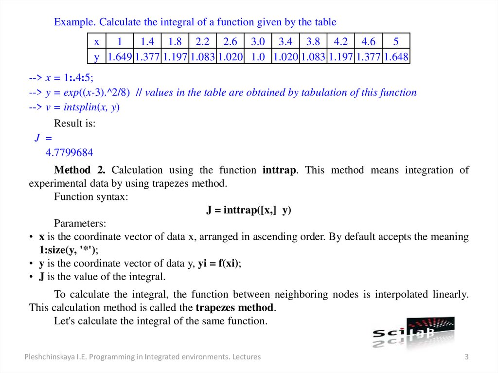
Example. Calculate the integral of a function given by the table
x
1
1.4 1.8 2.2 2.6 3.0 3.4 3.8 4.2 4.6
5
y 1.649 1.377 1.197 1.083 1.020 1.0 1.020 1.083 1.197 1.377 1.648
--> x = 1:.4:5;
--> y = exp((x-3).^2/8) // values in the table are obtained by tabulation of this function
--> v = intsplin(x, y)
Result is:
J =
4.7799684
Method 2. Calculation using the function inttrap. This method means integration of
experimental data by using trapezes method.
Function syntax:
J = inttrap([x,] y)
Parameters:
• x is the coordinate vector of data x, arranged in ascending order. By default accepts the meaning
1:size(y, '*');
• y is the coordinate vector of data y, yi = f(xi);
• J is the value of the integral.
To calculate the integral, the function between neighboring nodes is interpolated linearly.
This calculation method is called the trapezes method.
Let's calculate the integral of the same function.
Pleshchinskaya I.E. Programming in Integrated environments. Lectures
3

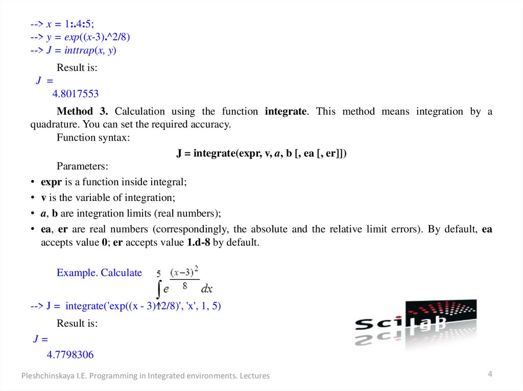
4.

--> x = 1:.4:5;
--> y = exp((x-3).^2/8)
--> J = inttrap(x, y)
Result is:
J =
4.8017553
Method 3. Calculation using the function integrate. This method means integration by a
quadrature. You can set the required accuracy.
Function syntax:
J = integrate(expr, v, a, b [, ea [, er]])
Parameters:
• expr is a function inside integral;
• v is the variable of integration;
• a, b are integration limits (real numbers);
• ea, er are real numbers (correspondingly, the absolute and the relative limit errors). By default, ea
accepts value 0; er accepts value 1.d-8 by default.
Example. Calculate
--> J = integrate('exp((x - 3)^2/8)', 'x', 1, 5)
Result is:
J=
4.7798306
Pleshchinskaya I.E. Programming in Integrated environments. Lectures
4

5.

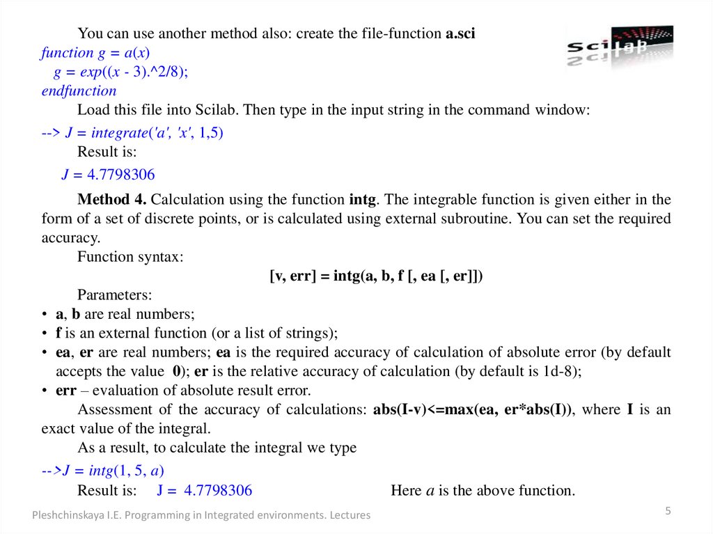
You can use another method also: create the file-function a.sci
function g = a(x)
g = exp((x - 3).^2/8);
endfunction
Load this file into Scilab. Then type in the input string in the command window:
--> J = integrate('a', 'x', 1,5)
Result is:
J = 4.7798306
Method 4. Calculation using the function intg. The integrable function is given either in the
form of a set of discrete points, or is calculated using external subroutine. You can set the required
accuracy.
Function syntax:
[v, err] = intg(a, b, f [, ea [, er]])
Parameters:
• a, b are real numbers;
• f is an external function (or a list of strings);
• ea, er are real numbers; ea is the required accuracy of calculation of absolute error (by default
accepts the value 0); er is the relative accuracy of calculation (by default is 1d-8);
• err – evaluation of absolute result error.
Assessment of the accuracy of calculations: abs(I-v)<=max(ea, er*abs(I)), where I is an
exact value of the integral.
As a result, to calculate the integral we type
-->J = intg(1, 5, a)
Result is: J = 4.7798306
Here a is the above function.
Pleshchinskaya I.E. Programming in Integrated environments. Lectures
5

6. Solution of the Cauchy problem for ordinary differential equations of the first order

Statement of the Cauchy problem: find a solution of an ordinary differential equation (ODE)
of the first order, written down in canonical form,
satisfying the initial condition
To solve this problem in the simplest case, you can use the ode function of the following
syntax:
y=ode(y0, x0, x, f).
Parameters:
• y is the vector of the values of the solution;
• x0, y0 is the initial value;
• x is a vector of arguments values for which the solution is being constructed;
• f is the external function determining the right side of the equation.
Example. Solve the Cauchy problem:
step h = 1.
on the segment [1, 10] with
Write down the equation in the canonical form: (i.e. in our case
an external function by using the file-function and apply the ode function:
Pleshchinskaya I.E. Programming in Integrated environments. Lectures
) Set
6

7.

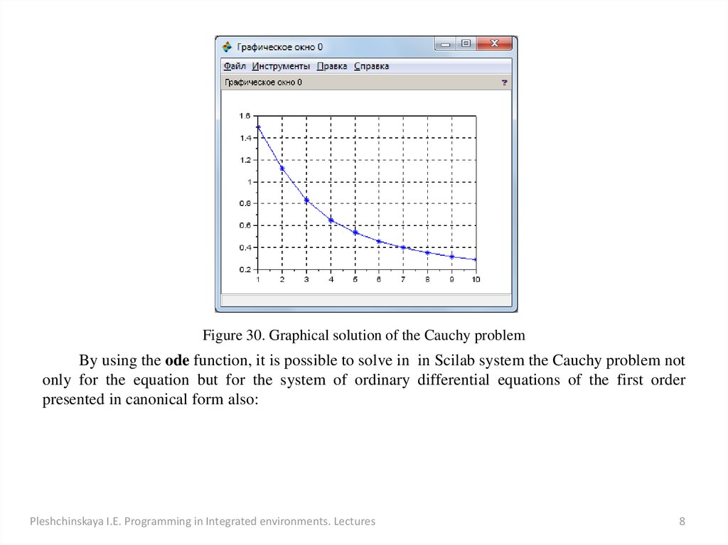
function w = f(x, y) // right side of equation
w = -y + sin(x*y);
endfunction
clc
scf
format('v', 5) // to reduce the number of displayed decimal places
x0 = 1;
y0 = 1.5;
x = [1:10]; // values of argument
z = ode(y0, x0, x, f); // the values you want to find of the solution of the Cauchy problem
plot(x, z, '-*'); xgrid() // graph of integral curve (of solution of ODE)
// by asterisks the values of solution at fixed points of the interval [1, 10] are denoted
The graphical result of this solution is represented on picture 30.
To get in the command window the numerical solution of the Cauchy problem it is sufficient
to remove the semicolon in the text of the program at the end of the line x = [1:10]; and of the line
z=ode(y0, x0, x, f);.
Result is:
x = 1.
2.
3.
z = 1.5 1.12 0.83
4.
0.65
5.
6.
0.54 0.46
7.
8.
9.
10.
0.40 0.35 0.32 0.29
Pleshchinskaya I.E. Programming in Integrated environments. Lectures
7

8.

Figure 30. Graphical solution of the Cauchy problem
By using the ode function, it is possible to solve in in Scilab system the Cauchy problem not
only for the equation but for the system of ordinary differential equations of the first order
presented in canonical form also:
Pleshchinskaya I.E. Programming in Integrated environments. Lectures
8

9.

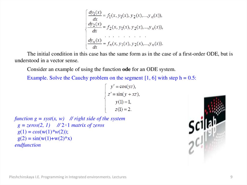
The initial condition in this case has the same form as in the case of a first-order ODE, but is
understood in a vector sense.
Consider an example of using the function ode for an ODE system.
Example. Solve the Cauchy problem on the segment [1, 6] with step h = 0.5:
function g = syst(x, w) // right side of the system
g = zeros(2, 1) // 2×1 matrix of zeros
g(1) = cos(w(1)*w(2));
g(2) = sin(w(1)+w(2)*x)
endfunction
Pleshchinskaya I.E. Programming in Integrated environments. Lectures
9

10.

clc, scf
format('v', 5) // to reduce the number of displayed decimal places
w0 = [1; 2]; x0 = 1;
x = [1:0.5:6] // values of argument
w = ode(w0, x0, x, syst) // the values you want to find of the solution of the Cauchy problem
plot(x, w, '-*'); xgrid(), legend('y', 'z', 2) // graphics of integral curves
Figure 31. Graphical solution of the Cauchy problem for the ODE system
Pleshchinskaya I.E. Programming in Integrated environments. Lectures
10

11.

The result of the numerical solution:
x=
1. 1.5
2. 2.5
3.
3.5
4. 4.5
5. 5.5
6.
w=
1. 0.88
2. 1.88
0.90 1.04
1.55 1.17
1.25
0.84
1.53 1.87 2.26 2.71 3.19 3.69
0.59 0.4 0.25 0.13 0.03 - 0.06
Here w = [w(1), w(2)] [y, z].
In general case, the ode function has the following syntax:
[y, w, iw]=ode([type], y0, x0, x, [, rtol [, atol]], f [, jak] [, w, iw]).
The required parameters y0, x0, x, f, y are described above. Consider some other parameters
of the ode function:
• type is a parameter to select the method of solution or the problem type: adams is a method of
forecasting-correcting of Adams; stiff is a method for solving hard problems; rk is the RungeKutta method of order 4; rkf is a five-step method of 4-th order; fix is the same Runge-Kutta
method with fixed increment;
• rtol, atol are the relative and the absolute calculating errors, i.e. a vector, which has the same
dimension as the dimension of the solution vector, y; by default, rtol = 0.00001, atol =
0.0000001, if you use the rkf and fix, rtol, atol = 0.001 = 0.0001;
• jak is a matrix that represents the right part of the Jacobian of rigid ODE system, usually
specify the matrix as the external functions of the form J = jak (x, y);
• w, iw are vectors, designed to store information on parameters of integration, which are applyed
to make subsequent calculations with the same parameters.
Pleshchinskaya I.E. Programming in Integrated environments. Lectures
11

12. Linear programming problems

Linear programming problems are the problems of the multidimensional optimization, in
which the criterion function is linear relative to their arguments and all restrictions on these
arguments have the form of linear equations and inequalities:
For solving linear programming problems in the Scilab system you should use different
built-in functions in dependence on the version of the framework. For example, in the Scilab 4.1.2
linear programming problem of the form
by conditions:
solves function linpro of the following syntax:
[x, lagr, f]=linpro(p, A, b, ci, cs, me [,x0])
Parameters:
x = (x1, x2, ... , xn) is a vector of the optimal values;
p'*x = f*x is the minimum value of the criterion function;
A1*x = b1 are restrictions-equalities;
A2*x< = b2 are restrictions-inequalities;
A=[A1; A2] is the matrix coefficients of the left parts of restrictions;
b=[b1; b2] is the vector of the right parts of restrictions;
Pleshchinskaya I.E. Programming in Integrated environments. Lectures
12

13.

• ci, cs are vectors respectively of the lower and of the upper bounds for x, i.e. ci <= x <= cs;
• me is the number of restrictions-equalities;
• x0='v'.
Linpro function returns the vector of unknown values of x, the minimum value of the
criterion function f and an array of Lagrange multipliers.
Note. If the problem is not to find the min(f), but the max(f), it is advisable to look for a
solution in the form of
[x, lagr, f] = linpro(p1, A, b, ci, cs, me [,x0])), f1
where f1=-f, p1=-p.
An example of solving transport problem: the city has three warehouses of flour and two
of the bakery. Daily 80 tons of flour is delivered to the 1-st bakery, and 70 t is delivered to the 2nd bakery. By this 50 tons are exported each day from the 1-st warehouse, 60 tons are exported
each day from the 2-nd warehouse, and 40 t from the 3-rd. The cost of transporting a ton of flour
from each warehouse is known:
• 300 rubles – for transport from the 1-st warehouse to the 1-st bakery;
• 200 rubles – for transport from the 1-st warehouse to the 2-nd bakery;
• 200 rubles – for transport from the 2-nd warehouse to the 1-st bakery;
• 350 rubles – for transport from the 2-nd warehouse to the 2-nd bakery;
• 250 rubles – for transport from the 3-rd warehouse to the 1-st bakery;
• 400 rubles – for transport from the 3-rd warehouse to the 2-nd bakery.
How to plan a shipment of flour, to minimize transport costs?
Pleshchinskaya I.E. Programming in Integrated environments. Lectures
13

14.

Let us construct a mathematical model of the transport problem. We will designate the
quantity of a flour transported daily from the 1-st warehouse to the 1-st bakery through
, from
the 1-st warehouse to the 2-nd bakery through , from the 2-nd warehouse to the 1-st bakery
through , from the 2-nd warehouse to the 2-nd bakery through , from the 3-rd warehouse to
the 1-st bakery through , from the 3-rd warehouse to the 2-nd bakery through
.
Then
The fact that a flour is delivered only from stores to bakeries but not in the opposite
direction, should be noted in our model as follows:
The cost of all the traffic
(criterion function) in our notations has the following form:
Obviously, it is necessary to look for min f(x).
To solve this problem in the Scilab 4.1.2 it is appropriate to use Editor window.
// Transport problem
// min(300x1 + 200x2 + 200x3 + 350x4 + 250x5 + 400x6)
// x1 + x2 = 50, x3 + x4 = 60, x5 + x6 = 40
// x1 + x3 + x5 = 80, x2 + x4 + x6 = 70
// x1>=0, x2>=0, x3>=0, x4>=0, x5>=0, x6>=0
clc
p = [300; 200; 200; 350; 250; 400];
Pleshchinskaya I.E. Programming in Integrated environments. Lectures
14

15.

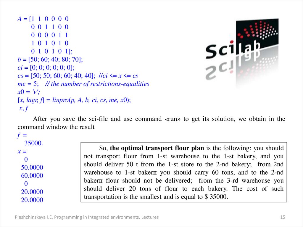
A = [1 1 0 0 0 0
0 0 1 1 0 0
0 0 0 0 1 1
1 0 1 0 1 0
0 1 0 1 0 1];
b = [50; 60; 40; 80; 70];
ci = [0; 0; 0; 0; 0; 0];
cs = [50; 50; 60; 60; 40; 40]; //ci <= x <= cs
me = 5; // the number of restrictions-equalities
x0 = 'v';
[x, lagr, f] = linpro(p, A, b, ci, cs, me, x0);
x, f
After you save the sci-file and use command «run» to get its solution, we obtain in the
command window the result
f =
35000.
So, the optimal transport flour plan is the following: you should
x=
not transport flour from 1-st warehouse to the 1-st bakery, and you
0
should deliver 50 t from the 1-st store to the 2-nd bakery; from 2nd
50.0000
warehouse to 1-st bakerн you should carry 60 tons, and to the 2-nd
60.0000
bakerн flour should not be delivered; from the 3-rd warehouse you
0
should deliver 20 tons of flour to each bakery. The cost of such
20.0000
transportation is the smallest and is equal to $ 35000.
20.0000
Pleshchinskaya I.E. Programming in Integrated environments. Lectures
15

16.

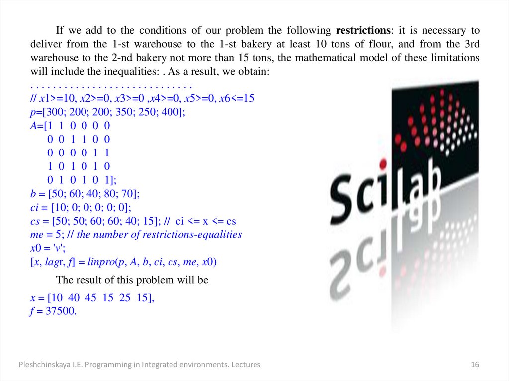
If we add to the conditions of our problem the following restrictions: it is necessary to
deliver from the 1-st warehouse to the 1-st bakery at least 10 tons of flour, and from the 3rd
warehouse to the 2-nd bakery not more than 15 tons, the mathematical model of these limitations
will include the inequalities: . As a result, we obtain:
.............................
// x1>=10, x2>=0, x3>=0 ,x4>=0, x5>=0, x6<=15
p=[300; 200; 200; 350; 250; 400];
A=[1 1 0 0 0 0
0 0 1 1 0 0
0 0 0 0 1 1
1 0 1 0 1 0
0 1 0 1 0 1];
b = [50; 60; 40; 80; 70];
ci = [10; 0; 0; 0; 0; 0];
cs = [50; 50; 60; 60; 40; 15]; // ci <= x <= cs
me = 5; // the number of restrictions-equalities
x0 = 'v';
[x, lagr, f] = linpro(p, A, b, ci, cs, me, x0)
The result of this problem will be
x = [10 40 45 15 25 15],
f = 37500.
Pleshchinskaya I.E. Programming in Integrated environments. Lectures
16

17.

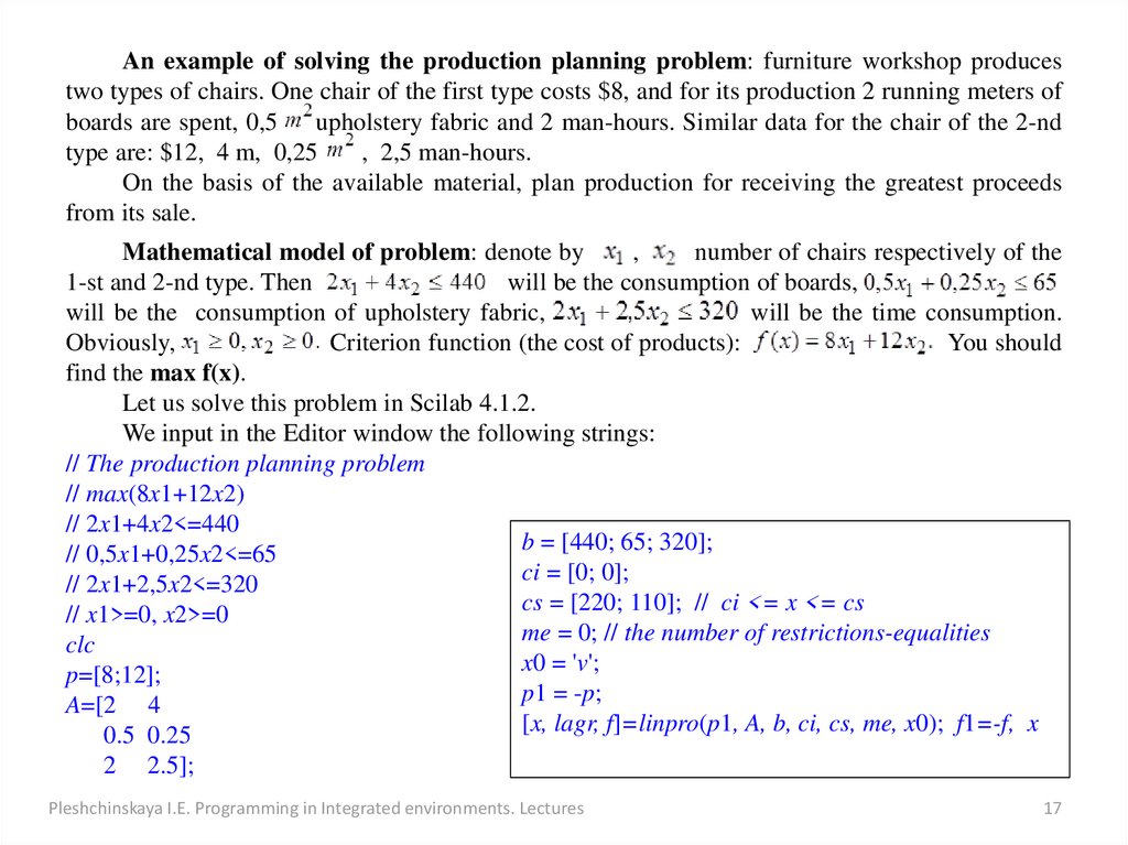
An example of solving the production planning problem: furniture workshop produces
two types of chairs. One chair of the first type costs $8, and for its production 2 running meters of
boards are spent, 0,5
upholstery fabric and 2 man-hours. Similar data for the chair of the 2-nd
type are: $12, 4 m, 0,25
, 2,5 man-hours.
On the basis of the available material, plan production for receiving the greatest proceeds
from its sale.
Mathematical model of problem: denote by
,
number of chairs respectively of the
1-st and 2-nd type. Then
will be the consumption of boards,
will be the consumption of upholstery fabric,
will be the time consumption.
Obviously,
Criterion function (the cost of products):
You should
find the max f(x).
Let us solve this problem in Scilab 4.1.2.
We input in the Editor window the following strings:
// The production planning problem
// max(8x1+12x2)
// 2x1+4x2<=440
b = [440; 65; 320];
// 0,5x1+0,25x2<=65
ci = [0; 0];
// 2x1+2,5x2<=320
cs = [220; 110]; // ci <= x <= cs
// x1>=0, x2>=0
me = 0; // the number of restrictions-equalities
clc
x0 = 'v';
p=[8;12];
p1 = -p;
A=[2 4
[x, lagr, f]=linpro(p1, A, b, ci, cs, me, x0); f1=-f, x
0.5 0.25
2 2.5];
Pleshchinskaya I.E. Programming in Integrated environments. Lectures
17

18.

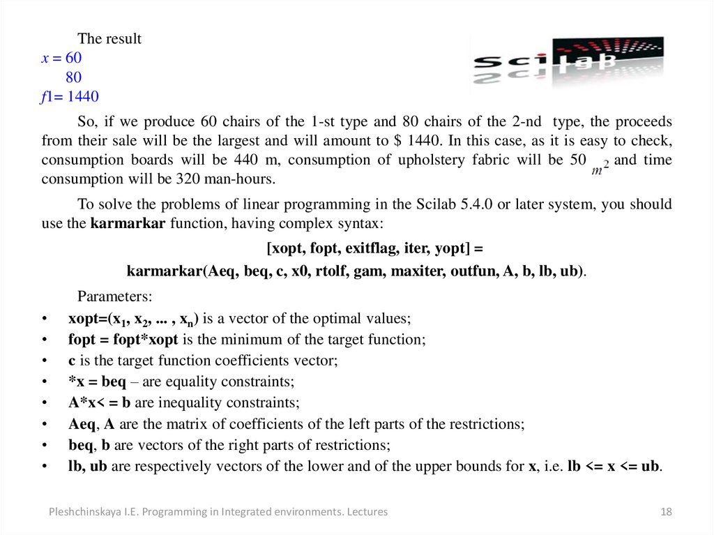
The result
x = 60
80
f1= 1440
So, if we produce 60 chairs of the 1-st type and 80 chairs of the 2-nd type, the proceeds
from their sale will be the largest and will amount to $ 1440. In this case, as it is easy to check,
consumption boards will be 440 m, consumption of upholstery fabric will be 50
and time
consumption will be 320 man-hours.
To solve the problems of linear programming in the Scilab 5.4.0 or later system, you should
use the karmarkar function, having complex syntax:
[xopt, fopt, exitflag, iter, yopt] =
karmarkar(Aeq, beq, c, x0, rtolf, gam, maxiter, outfun, A, b, lb, ub).
Parameters:
xopt=(x1, x2, ... , xn) is a vector of the optimal values;
fopt = fopt*xopt is the minimum of the target function;
с is the target function coefficients vector;
*x = beq – are equality constraints;
A*x< = b are inequality constraints;
Aeq, A are the matrix of coefficients of the left parts of the restrictions;
beq, b are vectors of the right parts of restrictions;
lb, ub are respectively vectors of the lower and of the upper bounds for x, i.e. lb <= x <= ub.
Pleshchinskaya I.E. Programming in Integrated environments. Lectures
18

19.

Note 1. Above not all parameters of function karmarkar are indicated, but only the most
important ones. The appointment of the remaining input and output parameters the user can find
by himself using the help system of the environment
.
Note 2. You can use the function karmarkar of a simplified form
[xopt, fopt]=karmarkar(Aeq, beq, c, [ ], [ ], [ ], [ ], [ ], A, b, lb, ub).
In the case when linear programming problem has no restrictions-equalities or restrictionsinequalities, you should by call of the function karmarkar specify these input parameters as [].
Let us solve the previous problem in Scilab 5.4.0.
We input in the Editor window the following strings:
// The production planning problem
// max (8x1+12x2)
// 2x1+4x2<=440
// 0,5x1+0,25x2<=65
// 2x1+2,5x2<=320
// x1>=0, x2>=0
clc
lb = [0; 0];
ub = [220; 110]; // lb <= x <= ub
c=[8;12];
me = 0; // the number of restrictions-equalities
A=[2 4
c1 = -c;
0.5 0.25
[xopt, fopt] = karmarkar ([], [], c1, [], [], [], [], [], A, b, lb, ub);
2 2.5];
fopt = - fopt; xopt, fopt
b = [440; 65; 320];
Pleshchinskaya I.E. Programming in Integrated environments. Lectures
19

20.

The result is
x = 60
80
fopt = 1440
As you see, the results of solving this linear programming problem using linpro function in
Scilab 4.1.2 and karmarkar function in Scilab 5.4.0 coincide.
Comparison of the results of solving the same linear programming problems using linpro
function in Scilab 4.1.2 and karmarkar function in Scilab 5.4.0 showed that in some cases the
results do not coincide. This is due to the specificity of optimization problems (their solution is
not always the unique) and to the differences of functions linpro and karmarkar.
Note 3. In order to have opportunity to solve problems of linear programming in the Scilab
5.4.0 using the linpro function, one should use special additional utility quapro by
downloading it from the website http://atoms.scilab.org/toolboxes/quapro.
Pleshchinskaya I.E. Programming in Integrated environments. Lectures
20