


 Информатика
 Электроника
Похожие презентации:


")


DCT – Wavelet – Filter Bank
1. DCT – Wavelet – Filter Bank
Trac D.TranDepartment of Electrical and Computer Engineering
The Johns Hopkins University
Baltimore, MD 21218
2. Outline
ReminderLinear signal decomposition
Optimal linear transform: KLT, principal component analysis
Discrete cosine transform
Definition, properties, fast implementation
Review of multi-rate signal processing
Wavelet and filter banks
Aliasing cancellation and perfect reconstruction
Spectral factorization: orthogonal, biorthogonal, symmetry
Vanishing moments, regularity, smoothness
Lattice structure and lifting scheme
M-band design – Local cosine/sine bases
3.
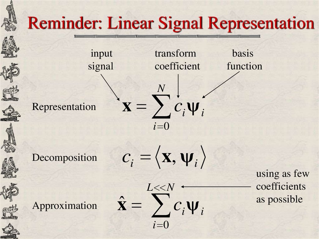
Reminder: Linear Signal Representationinput
signal
transform
coefficient
basis
function
N
Representation
x ci ψ i
i 0
Decomposition
Approximation
ci x, ψ i
xˆ
using as few
coefficients
as possible
L N
c ψ
i 0
i
i
4. Motivations
Fundamental question: what is the best basis?energy compaction: minimize a pre-defined error measure, say
MSE, given L coefficients
maximize perceptual reconstruction quality
low complexity: fast-computable decomposition and
reconstruction
intuitive interpretation
How to construct such a basis? Different viewpoints!
Applications
compression, coding
signal analysis
de-noising, enhancement
communications
5. KLT: Optimal Linear Transform
R xx Φi i ΦiT
E xx
KLT Φ 0
eigenvectors
Φ1
Φ N 1
Signal dependent
Require stationary signals
How do we communicate bases to the decoder?
How do we design “good” signal-independent transform?
6. Discrete Cosine Transforms
Type IC
2
M
I
C
III
Type IV
C
IV
2
M
,
m, n 0,1, , M
2
M
m n 1 2
K m cos
M
,
m, n 0,1, , M 1
2
M
m 1 2 n
K n cos
M
,
m, n 0,1, , M 1
m 1 2 n 1 2
cos
M
,
m, n 0,1, , M 1
Type III
C
mn
K m K n cos M
Type II
II
1 2 , i 0, M
Ki
otherwise
1,
7. DCT Type-II
1,
Ki 2
1,
8 x 8 block
i 0 DC
i 0
orthogonal
real coefficients
symmetry
near-optimal
fast algorithms
horizontal edges
DCT basis
M 1
2
(2n 1)m
x[n] cos
X [ m]
K
m
M
2M
n 0
M 1
(2m 1)n
x[n] 2
X
[
m
]
cos
K
n
M
2M
m 0
m, n 0,1,..., M 1
vertical edges
8. DCT Symmetry
m 2 M 1 n 1cos
2M
2 M 2 2n 1 m
cos
2M
2 Mm 2n 1 m
cos
2M
2M
2n 1 m
cos
2M
DCT basis functions
are either symmetric
or anti-symmetric
9. DCT: Recursive Property
An M-point DCT–II can be implemented via an M/2-pointDCT–II and an M/2-point DCT–IV
C
II
M
II
1 CM/2
2 0
0 I J
IV
CM/2 J J I
Butterfly
CIIM/2
DCT
coefficients
input
samples
C
IV
M/2
J
10. Fast DCT Implementation
13 multiplications and 29 additions per 8 input samples11. Block DCT
X1 CIIMX
2 0
X N
output blocks
of DCT coefficients,
each of size M
0
C
II
M
0
0
CIIM
0
x1
x2
0
II
C M x N
input blocks,
each of size M
12. Filtering
x[n]h[n]
y[n] h[n k ]x[k ] h[k ]x[n k ]
y[n]
k
k
y[n 1] h[2] h[1] h[0] 0
0
y[n] 0 h[2] h[1] h[0] 0
y
[
n
1
]
0 h[2] h[1] h[0]
0
x
[
n
2
]
x[n 1]
x
[
n
]
x[n 1]
X e j
n
Fourier :
H (e j ) h[ n]e j n
n
LTI Operator
z Transform : H ( z ) h[n] z n
H e j
Y e j X e j H e j
13. Down-Sampling
x[n ]2
y[n] x[2n]
x
[
1
]
y[ 1] 1 0 0 0 0
x[0]
y[0] 0 0 1 0 0
x[1]
y[1] 0 0 0 0 1 x[2]
Linear Time-Variant Lossy Operator
Y e j
X e j
2
1
Y e X e j / 2 X e j 2 / 2
2
1
Y z X z1/ 2 X z1/ 2
2
j
2
14. Up-Sampling
x[n ]2
x[n / 2], n even
y[n]
n odd
0,
1 0 0
y[ 1]
x[ 1]
0 0 0
y[0]
x[0]
0 1 0 x[1]
y[1] 0 0 0
y[2]
x[2]
0 0 1
Y e j
Y z X z 2
X e j
Y e j X e j 2
2
2
15. Filter Bank
First FB designed for speech coding, [Croisier-Esteban-Galand 1976]Orthogonal FIR filter bank, [Smith-Barnwell 1984], [Mintzer 1985]
low-pass filter
2
2
F0 ( z )
2
F1 ( z)
Q
H1 ( z )
2
high-pass filter
high-pass filter
Analysis Bank
Synthesis Bank
X ( e j )
2
2
X (z )
H 0 ( z)
low-pass filter
Xˆ ( z )
16. FB Analysis
X (z )H 0 ( z)
2
2
F0 ( z )
2
F1 ( z)
Q
H1 ( z )
2
Xˆ ( z )
for Distortion Eliminatio n, set to 2 z l
1
ˆ
X ( z ) F0 ( z ) H 0 ( z ) F1 ( z ) H1 ( z ) X ( z )
2
1
F0 ( z ) H 0 ( z ) F1 ( z ) H1 ( z ) X ( z )
2
for Aliasing Cancellati on, set to 0!
z l X ( z )
F0 ( z ) H1 ( z )
F1 ( z ) H 0 ( z )
Alternating-Sign Construction
17. Perfect Reconstruction
With Aliasing CancellationF0 ( z ) H1 ( z )
F1 ( z ) H 0 ( z )
Distortion Elimination becomes
F0 ( z ) H 0 ( z ) F0 ( z ) H 0 ( z ) 2 z l
P0 ( z ) P0 ( z ) 2 z l where P0 ( z ) F0 ( z ) H 0 ( z )
Half-band Filter
18. Half-band Filter
P0 ( z ) a bz 1 cz 2 dz 3 ez 4lone odd-power
P0 ( z ) a bz 1 cz 2 dz 3 ez 4
P0 ( z ) P0 ( z ) 0 2bz 1 0 2dz 3 0 2 z l
can only have one odd-power
Standard design procedure
Design a good low-pass half-band filter P0 ( z )
Factor P0 ( z ) into H 0 ( z ) and F0 ( z )
Use the aliasing cancellation condition to obtain H1 ( z ) and F1 ( z)
19. Spectral Factorization
multiplezeros
Im
z *
z and z* must stay together
z
z
*
Re
Orthogonality
f i [n] hi [ n]
1
Fi ( z ) H i ( z )
z and z^-1 must be separated
z 1
Symmetry
hi [n] hi [ L 1 n]
( L 1)
H i ( z) z
H i ( z 1 )
z and z^-1 must stay together
Zeros of Half-band Filter
P0 ( z ) (1 zn z 1 );
Real-coefficient
zn roots
n
H 0 ( z ) (1 zk z 1 )
k H
F0 ( z ) (1 zl z 1 )
l F
20. Spectral Factorization: Orthogonal
Imz
Im
z *
8 zeros
Minimum
Phase
4 zeros
z*
Re
z
z
*
Re
Im
z 1
4 zeros
Maximum
Phase
z *
Re
z 1
21. Spectral Factorization: Symmetry
z *Im
z
Im
8 zeros
z
*
9-tap H0
z
4 zeros
*
Re
z
z
*
z 1
Re
Im
z 1
4 zeros
7-tap F0
Re
22. History: Wavelets
Early wavelets: for geophysics, seismic, oil-prospectingapplications, [Morlet-Grossman-Meyer 1980-1984]
Compact-support wavelets with smoothness and regularity,
[Daubechies 1988]
Linkage to filter banks and multi-resolution representation,
fast discrete wavelet transform (DWT), [Mallat 1989]
Even faster and more efficient implementations: lattice
structure for filter banks, [Vaidyanathan-Hoang 1988];
lifting scheme, [Sweldens 1995]
23. From Filter Bank to Wavelet
[Daubechies 1988], [Mallat 1989]Constructed as iterated filter bank
Discrete Wavelet Transform (DWT): iterate FB on
the lowpass subband
x[n ]
frequency spectrum
0
/4 /2
x(t )
i
c
(
2
i ,k t k )
k i 0
24. 1-Level 2D DWT
inputimage
x[m, n]
LP
HP
LP
LL: smooth approximation
HP
LH: horizontal edges
LP
HL: vertical edges
HP
HH: diagonal edges
decompose rows decompose columns
L
LL
LH
HL
HH
H
25. 2-Level 2D DWT
LPLP
HP
LP
LP
HP
LP
HP
HP
HP
LP
decompose rows decompose columns
HP
decompose rows decompose columns
LH
HL
HH
26. 2D DWT
27. Time-Frequency Localization
x[n] cos( a n) [n]t
best time
localization
t
STFT
uniform tiling
t
wavelet
dyadic tiling
t
best frequency
localization
Heisenberg’s Uncertainty Principle: bound on T-F product
Wavelets provide flexibility and good time-frequency trade-off
28. Wavelet Packet
Iterate adaptively according to the signalArbitrary tiling of the time-frequency plain
x[n ]
frequency spectrum
0
/2
Question: can we iterate
any FB to construct wavelets
and wavelet packets?
29. Scaling and Wavelet Function
H 0 (z 4 )8
H1 ( z 4 )
8
H 0 (z 2 )
x[n ]
H 0 ( z)
H1 ( z 2 )
4
2
H1 ( z)
L
Discrete Basis
H ( z) H 0 ( z
L
0
k 1
i 1
2 k 1
)
product
filters
2 k 1
2i 1
H ( z ) H 0 ( z ) H 1 ( z )
k 1
i
1
Continuous-time Basis
scaling function
1
(
)
H
(t) 2 h0 [n] (2t n)
0 k
2
2
n
k 1
1
( ) 1 H
H
(t) 2 h1 [n] (2t n)
1
0 k
2 2 k 2 2
2
n
wavelet function
30. Convergence & Smoothness
Convergence & SmoothnessNot all FB yields nice product filters
Two fundamental questions
Will the infinite product converge?
Will the infinite product converge to a smooth function?
Necessary condition for convergence: at least a zero at
Sufficient condition for smoothness: many zeros at
with 2 zeros at
with 4 zeros at
31. Regularity & Vanishing Moments
Regularity & Vanishing MomentsIn an orthogonal filter bank, the scaling filter has K vanishing
moments (or is K-regular) if and only if
Scaling filter has K zeros at
k
k 0,1,..., K 1
n h1 [n] 0,
n
All polynomial sequences up to degree (K-1) can be
expressed as a linear combination of integer-shifted scaling
filters [Daubechies]
Design Procedure: max-flat half-band spectral factorization
P0 ( z ) 1 z
1 2 K
enforce the half-band condition here
Q( z )
maximize the number of vanishing moments
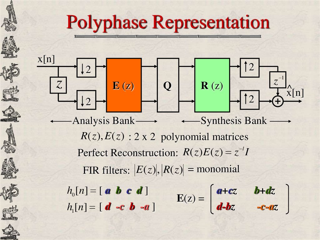
32.
Polyphase Representationx[n]
2
2
z
E (z)
Q
z 1
R (z)
2
2
Analysis Bank
Synthesis Bank
R( z ), E ( z ) : 2 x 2 polynomial matrices
l
Perfect Reconstruction: R( z ) E ( z ) z I
FIR filters: E ( z ) , R( z ) = monomial
h0 [n] [ a b c d ]
h1[n] [ d -c b -a ]
E(z) =
a+cz
d-bz
b+dz
-c-az
^
x[n]
33. Lattice Structure
cos iRi
sin i
Orthogonal Lattice
x[n]
sin i
cos i
2
2
1
0
z
z
z
1 i
Ri
1
i
Linear-Phase Lattice
x[n]
2
z
2
z
z
…
34. FB Design from Lattice Structure
Set of free parametersi
or
i
Modular construction, well-conditioned, nice built-in properties
Complete characterization: lattice covers all possible solutions
Unconstrained optimization
stopband attenuation
min
f i
regularity
i
combination
35. Lifting Scheme
x[n]2
P0 ( z )
z
U 0 ( z)
2
…
K
…
1/ K
E (z )
0
0 1 U i ( z ) 1
K
E( z)
1 Pi ( z ) 1
0 1 / K i 0
Example:
1
0
1
1
(
1
z
)
1
E( z) 4
1
(
1
z
)
1
0
1 2
1 1 3 1 1
h0 [n] , , , ,
8 4 4 4 8
1
1
h1[n] , 1,
2
2
36. Wavelets: Summary
Closed-form constructionFundamental properties - Advantages
Ψ( 2t)
Time Scaled :
Mother Wav elet : Ψ(t) Translatio n :
Ψ(t-k)
Time Scaled Translatio n : Ψ( 2t-k)
non-redundant orthonormal bases, perfect reconstruction
compact support is possible
basis functions with varying lengths with zoom capability
smooth approximation
fast O(n) algorithms
Connection to other constructions
filter bank and sub-band coding in signal compression
multi-resolution in computer vision
multi-grid methods in numerical analysis
successive refinement in graphics