Linear Algebra. Lecture 2

1.

Linear Algebra
Lecture 2
Solution Sets of Linear Systems.
Applications of Linear Systems.
Linear Independence.
Aidana Zhalgas
[email protected]

2.

Learning Objectives:
1. Solving Homogeneous Systems.
2. Solving Nonhomogeneous Systems.
3. Applications.
4. Represent Linear Independence of sets of vectors.

3.

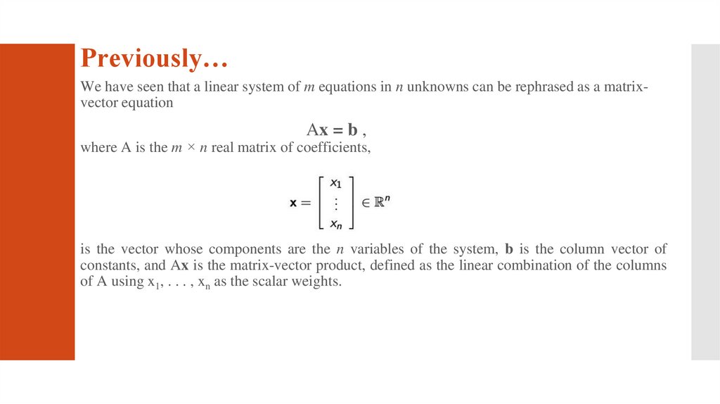
Previously…
We have seen that a linear system of m equations in n unknowns can be rephrased as a matrixvector equation
Ax = b ,
where A is the m × n real matrix of coefficients,
is the vector whose components are the n variables of the system, b is the column vector of
constants, and Ax is the matrix-vector product, defined as the linear combination of the columns
of A using x1, . . . , xn as the scalar weights.

4.

1.5. Solution Sets of Linear Systems.
Now we seek to understand the solution sets of such equations:
the hope is to be able to use the tools developed thus far to describe the set of all
x ∈ Rn satisfying a given equation Ax = b.
To do this, we turn first to the easiest case to study: the case when b = 0. Thus,
we are asking about linear combinations of the column vectors of A which equal
0, or equivalently, intersections of linear subsets of Rn that all pass through the
origin.
We will then discover that describing the solutions to Ax=0 help unlock a
general solution to Ax = b for any b.

5.

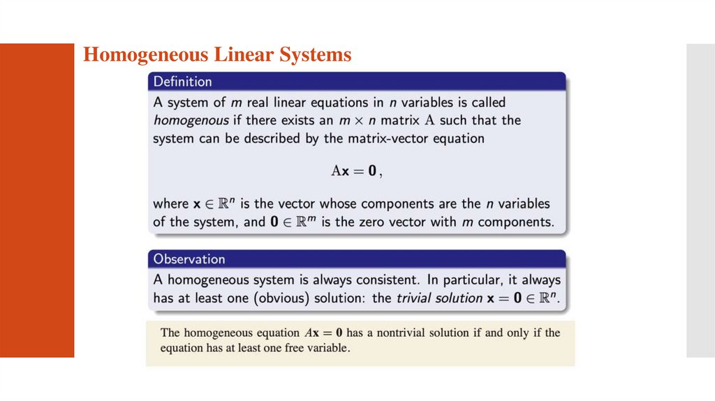
Homogeneous Linear Systems

6.

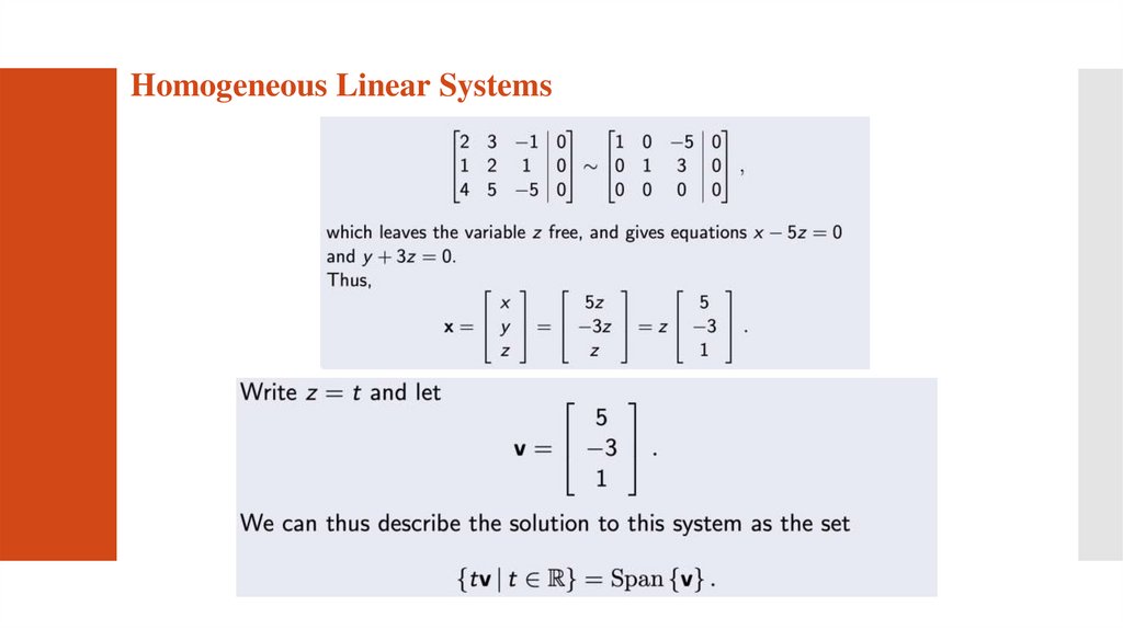
Homogeneous Linear Systems

7.

Homogeneous Linear Systems

8.

Homogeneous Linear Systems

9.

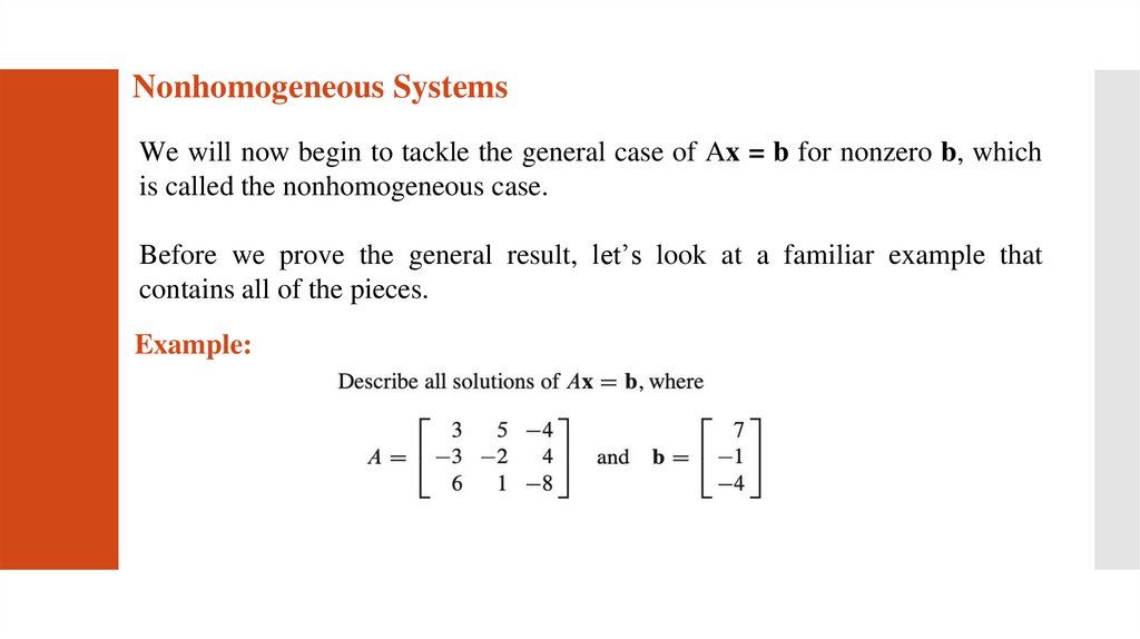
Nonhomogeneous Systems
We will now begin to tackle the general case of Ax = b for nonzero b, which
is called the nonhomogeneous case.
Before we prove the general result, let’s look at a familiar example that
contains all of the pieces.
Example:

10.

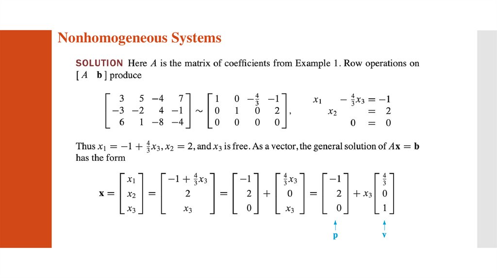
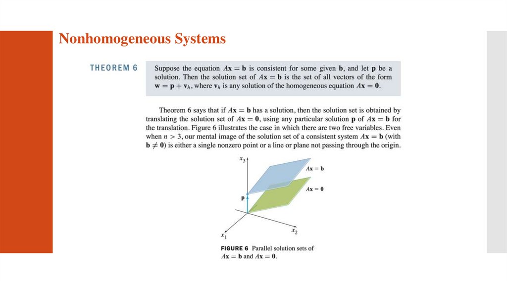
Nonhomogeneous Systems

11.

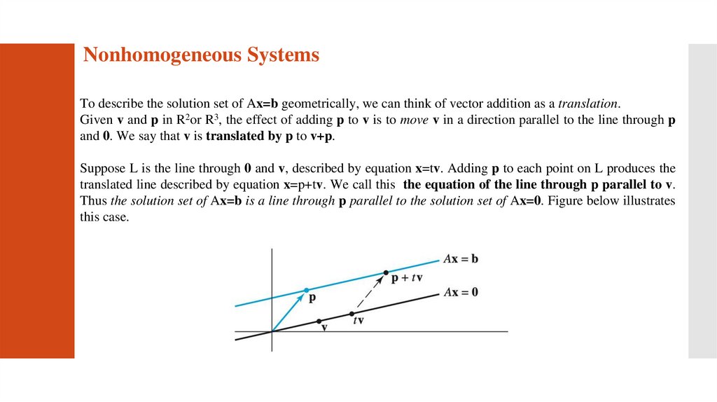
Nonhomogeneous Systems
To describe the solution set of Ax=b geometrically, we can think of vector addition as a translation.
Given v and p in R2or R3, the effect of adding p to v is to move v in a direction parallel to the line through p
and 0. We say that v is translated by p to v+p.
Suppose L is the line through 0 and v, described by equation x=tv. Adding p to each point on L produces the
translated line described by equation x=p+tv. We call this the equation of the line through p parallel to v.
Thus the solution set of Ax=b is a line through p parallel to the solution set of Ax=0. Figure below illustrates
this case.

12.

Nonhomogeneous Systems

13.

1.6. Applications of Linear Algebra in
SE
Any applications in software engineering where a large amount of equations need to be
calculated quickly, linear algebra is most likely being used. These applications would
include things like graphics software, visual gaming, physics, and signal processing.
Another application is in computer graphics. Using very simple linear algebra, as well as
parts of other branches of mathematics, you can easily make objects move around in a
virtual world, make them larger or smaller.
Web development hardly requires any knowledge of linear algebra. Building strong backends
to web frontends requires no knowledge of linear algebra (in most cases, randomization can
achieve good load balancing if you are building backend farms).

14.

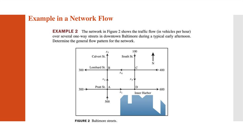
Example in a Network Flow
Urban planners and traffic engineers monitor the pattern of traffic flow in a grid of city streets.
Electrical engineers calculate current flow through electrical circuits. And economists analyze
the distribution of products from manufacturers to consumers through a network of
wholesalers and retailers. For many networks, the systems of equations involve hundreds or
even thousands of variables and equations.
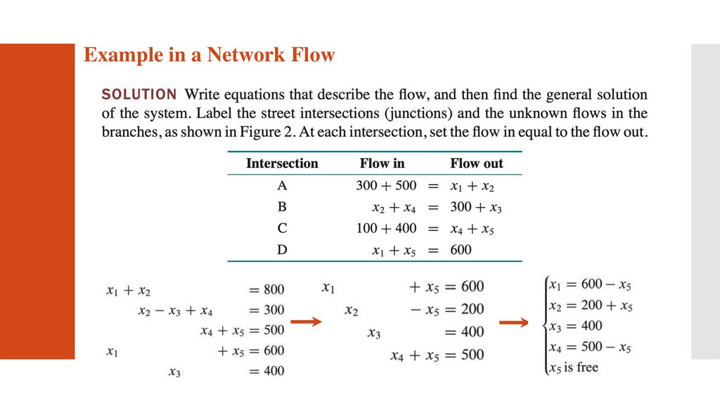
The basic assumption of network flow is that the total flow into the network equals the total
flow out of the network and that the total flow into a junction equals the total flow out of the
junction.

15.

Example in a Network Flow

16.

Example in a Network Flow

17.

1.7. Linear Independence

18.

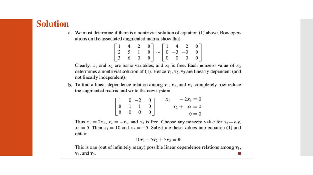
Solution

19.

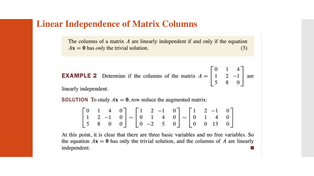
Linear Independence of Matrix Columns

20.

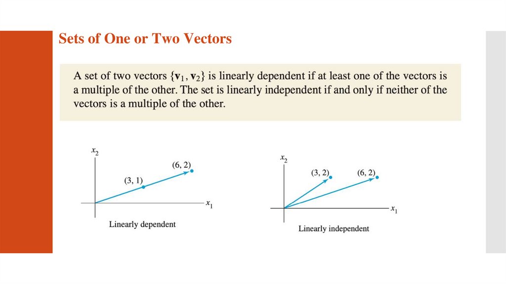
Sets of One or Two Vectors

21.

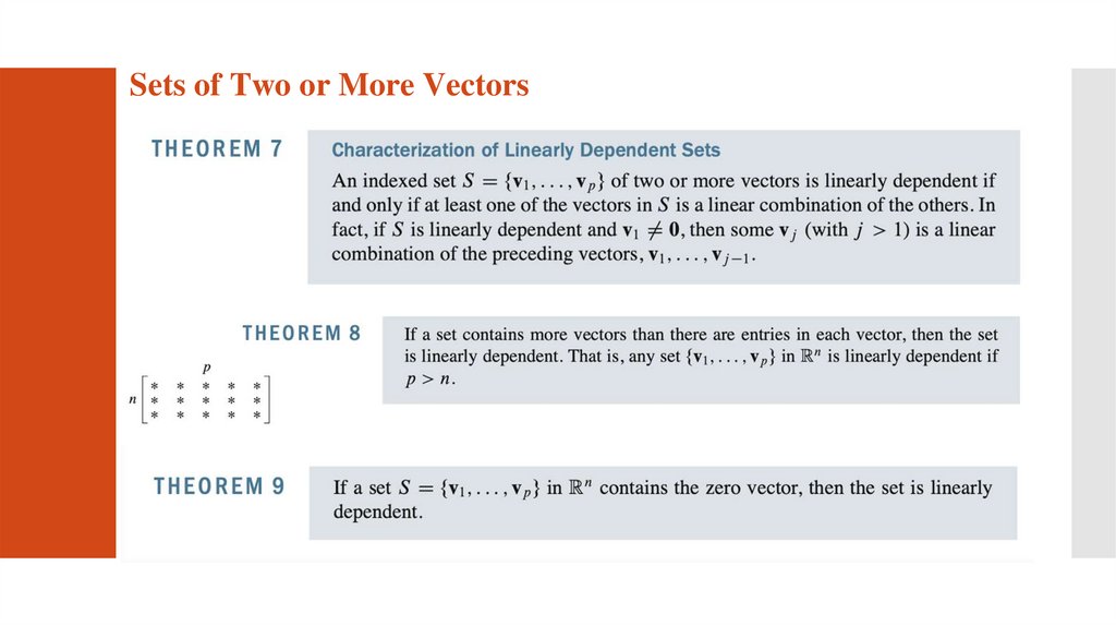
Sets of Two or More Vectors

22.

Lecture Summary
1.
2.
3.
Homogeneous and Nonhomogeneous Linear Systems (trivial/nontrivial solutions)
Applications
Linear Independence