Credit and exam

1.

Topics overview
Credit and exam

2.

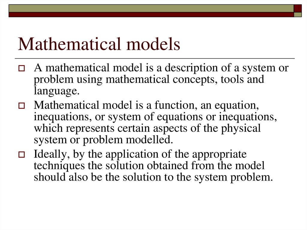
Mathematical models
A mathematical model is a description of a system or
problem using mathematical concepts, tools and
language.
Mathematical model is a function, an equation,
inequations, or system of equations or inequations,
which represents certain aspects of the physical
system or problem modelled.
Ideally, by the application of the appropriate
techniques the solution obtained from the model
should also be the solution to the system problem.

3.

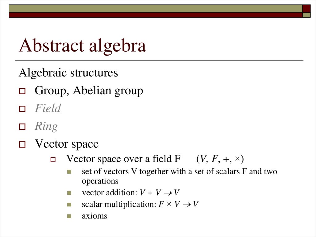
Abstract algebra
Algebraic structures
Group, Abelian group
Field
Ring
Vector space
Vector space over a field F
(V, F, +, ×)
set of vectors V together with a set of scalars F and two
operations
vector addition: V + V V
scalar multiplication: F × V V
axioms

4.

Linear algebra
Vector space
Vectors
Components (coordinates)
Basic operations
Linear combination of vectors
Linearly dependent or independent vectors
Basic types of vectors

5.

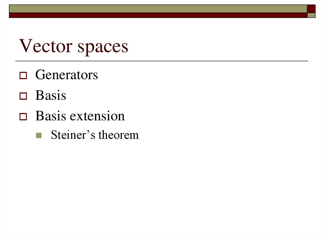
Vector spaces
Generators
Basis
Basis extension
Steiner’s theorem

6.

Matrices
Type of matrix
Matrix addition
Matrix multiplication
Scalar multiplication of matrix
Inversion of square matrix
Rank of matrix

7.

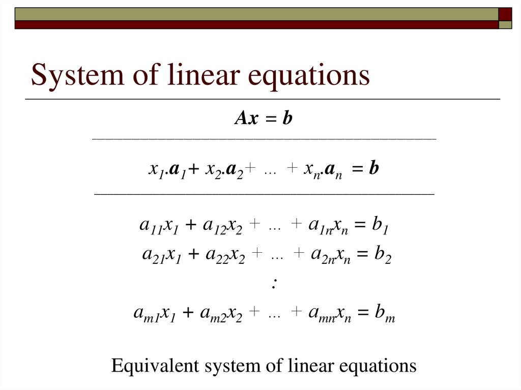
System of linear equations
Ax = b
_______________________________________________________________________________
x1.a1+ x2.a2+ … + xn.an = b
____________________________________________________
a11x1 + a12x2 + … + a1nxn = b1
a21x1 + a22x2 + … + a2nxn = b2
:
am1x1 + am2x2 + … + amnxn = bm
Equivalent system of linear equations

8.

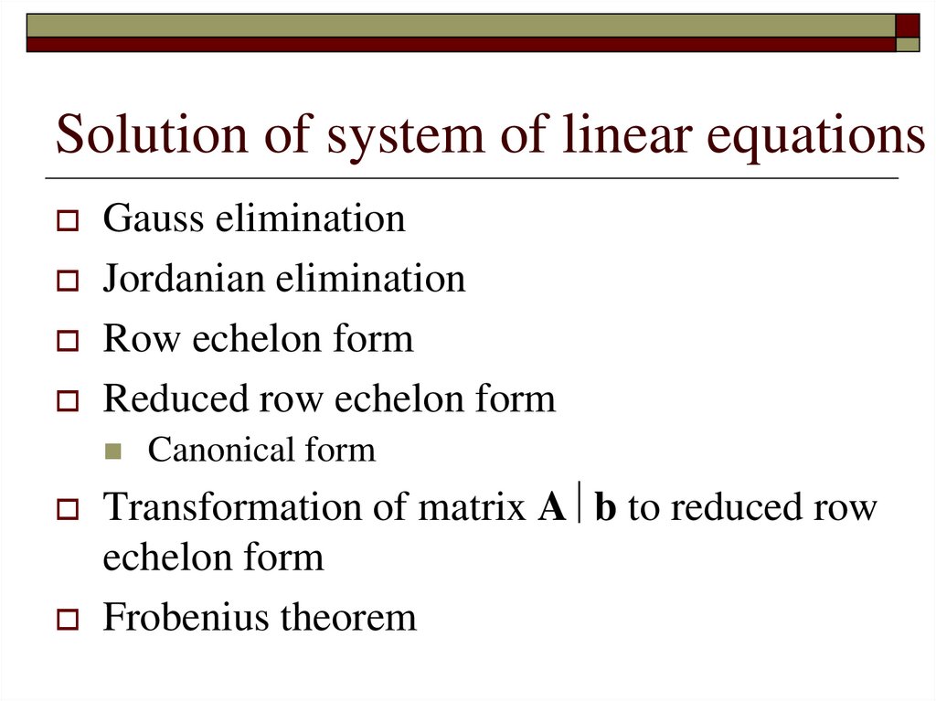
Solution of system of linear equations
Gauss elimination
Jordanian elimination
Row echelon form
Reduced row echelon form
Canonical form
Transformation of matrix A b to reduced row
echelon form
Frobenius theorem

9.

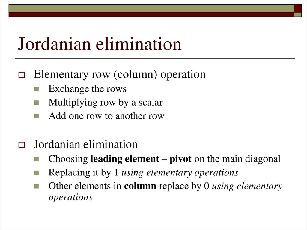
Jordanian elimination
Elementary row (column) operation
Exchange the rows
Multiplying row by a scalar
Add one row to another row
Jordanian elimination
Choosing leading element – pivot on the main diagonal
Replacing it by 1 using elementary operations
Other elements in column replace by 0 using elementary
operations

10.

Solubility of system of linear equations
The system has no solution (in this case, we say that
the system is overdetermined)
The system has a single solution (the system is exactly
determined)
The system has infinitely many solutions (the system
is underdetermined).
Basic solution
Nonbasic solution
Parametric solution

11.

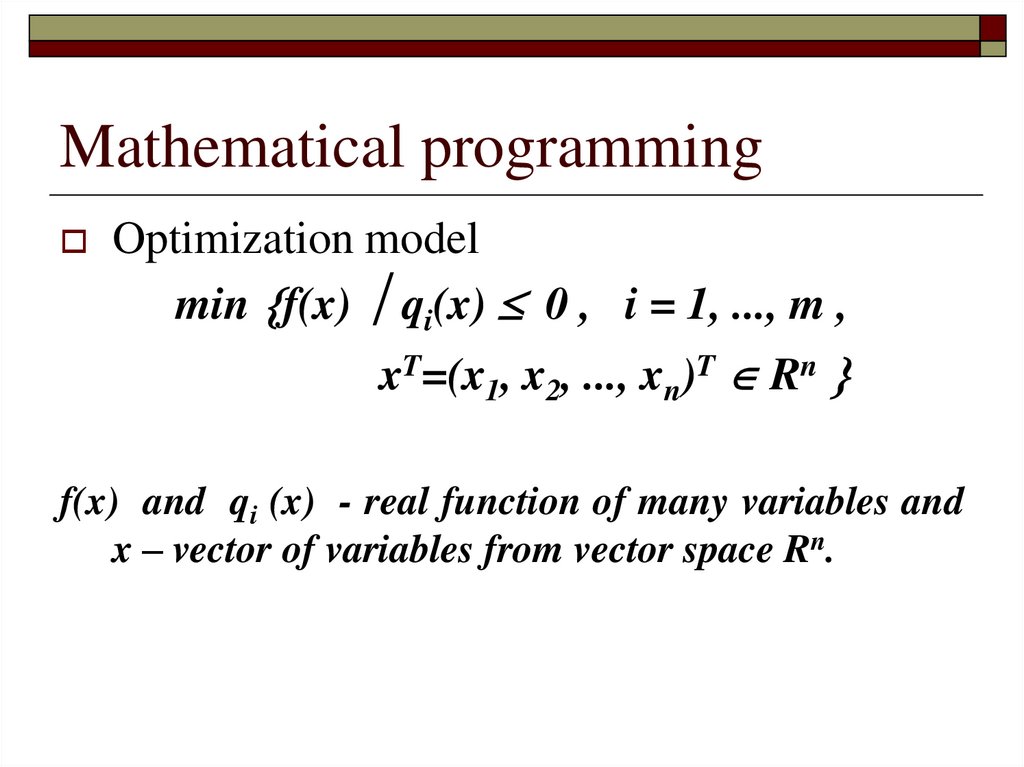
Mathematical programming
Optimization model
min f(x) qi(x) 0 , i = 1, ..., m ,
xT=(x1, x2, ..., xn)T Rn
f(x) and qi (x) - real function of many variables and
x – vector of variables from vector space Rn.

12.

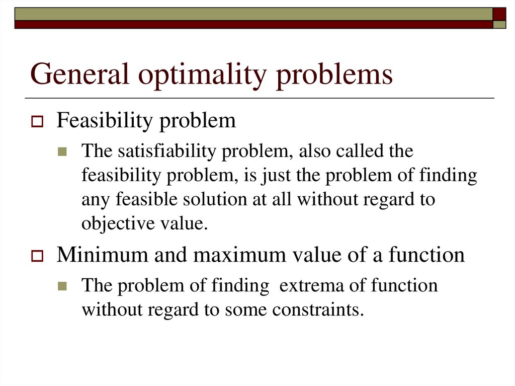
General optimality problems
Feasibility problem
The satisfiability problem, also called the
feasibility problem, is just the problem of finding
any feasible solution at all without regard to
objective value.
Minimum and maximum value of a function
The problem of finding extrema of function
without regard to some constraints.

13.

Classification of optimization models
More then one constraint
Number of criteria
Type of criteria
Single optimization
Multiple optimization
Minimization
Maximization
Goal problem
Type of functions
Linear model
Nonlinear model
Convex model
Nonconvex model

14.

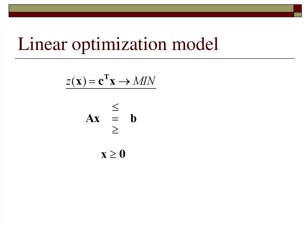
Linear optimization model
z (x) c T x MIN
Ax b
x 0

15.

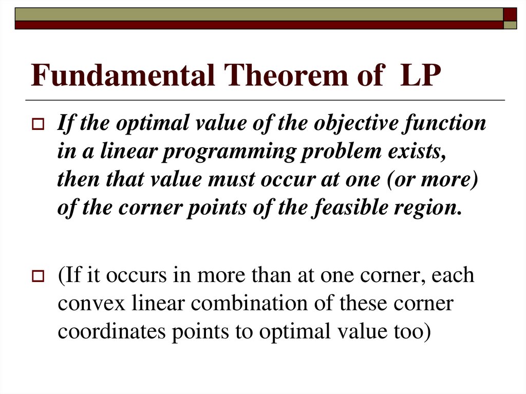
Fundamental Theorem of LP
If the optimal value of the objective function
in a linear programming problem exists,
then that value must occur at one (or more)
of the corner points of the feasible region.
(If it occurs in more than at one corner, each
convex linear combination of these corner
coordinates points to optimal value too)

16.

Fundamentals theorems
Basic solution of system of linear equations is
represented by corner points of the feasible
region.
If feasible solution of LP exists, basic feasible
solution exists too.
Optimal solution of LP problem lies on the
border of convex polytop of feasible solutions.
If optimal solution of LP exists, basic optimal
solution exists too.

17.

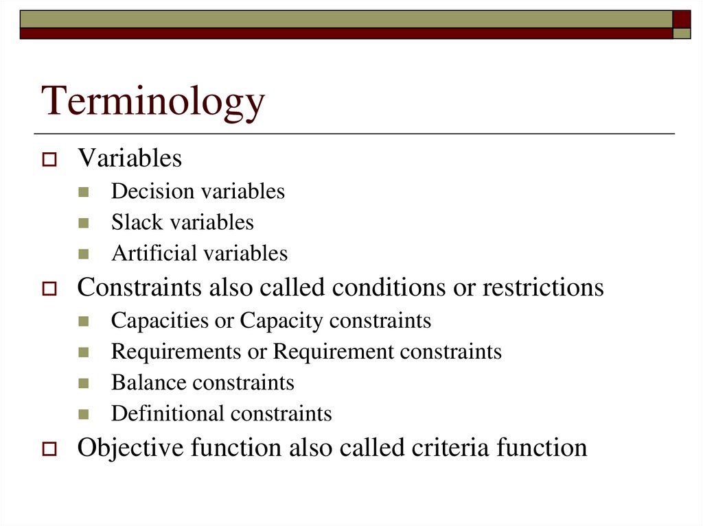
Terminology
Variables
Constraints also called conditions or restrictions
Decision variables
Slack variables
Artificial variables
Capacities or Capacity constraints
Requirements or Requirement constraints
Balance constraints
Definitional constraints
Objective function also called criteria function

18.

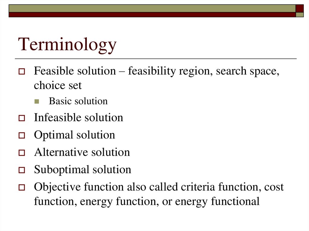
Terminology
Feasible solution – feasibility region, search space,
choice set
Basic solution
Infeasible solution
Optimal solution
Alternative solution
Suboptimal solution
Objective function also called criteria function, cost
function, energy function, or energy functional

19.

Existence of solution
Nonexistence of solution
If the feasible region is empty (that is, there are no points that
satisfy all the constraints), the both the maximum value and
the minimum value of the objective function do not exist.
If the feasible region is unbounded, and the vector of
coefficients of the objective function lies in the feasible cone,
then the minimum value of the objective function exists, but
the maximum value does not, is unbounded.
Existence of one or more solutions
If the feasible region for a linear programming problem is
bounded, then both the maximum value and the minimum
value of the objective function always exist.
If two or more optimal solutions exists, than infinite number
of solutions exist – linear combinations of some solution

20.

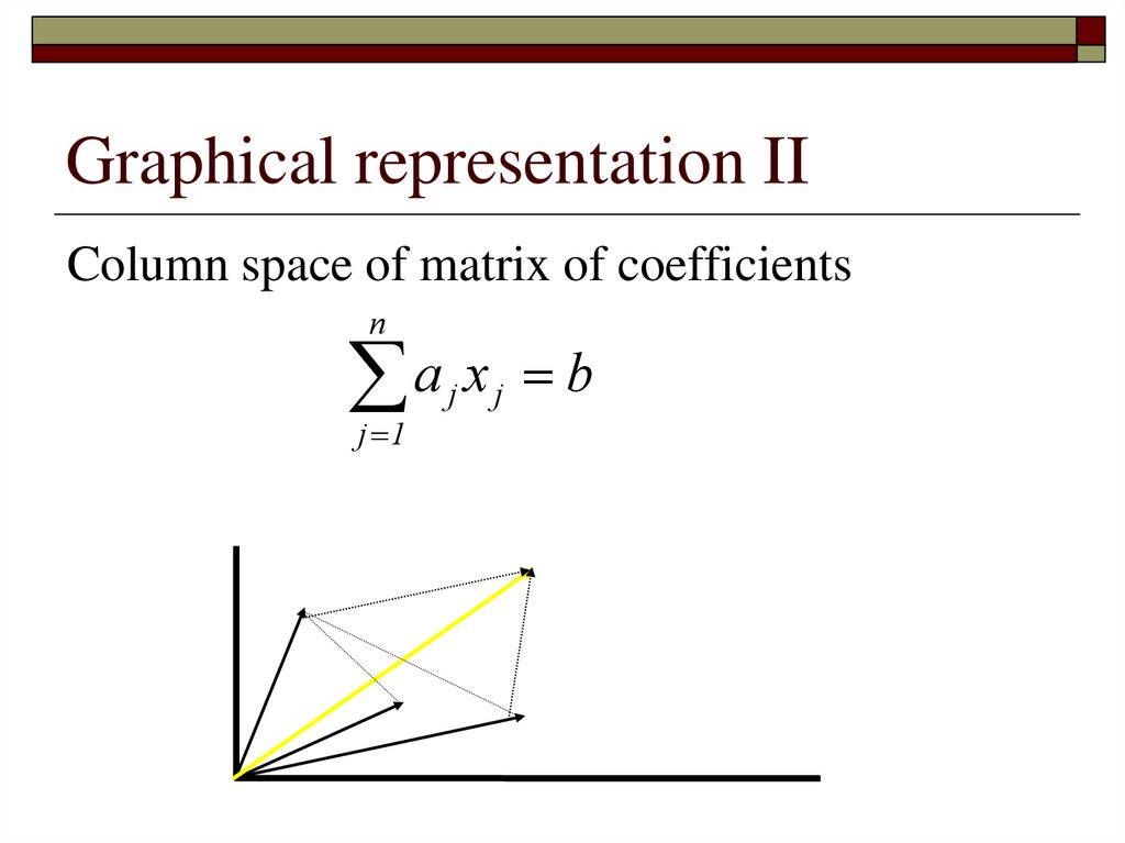
Matrices as basic vectors
Column space of a matrix is the set of all
possible linear combinations of its column
vectors
Description of vectors (Space of solutions)
Description of scalars (Column space)
Row space of a matrix is the set of all possible
linear combinations of its row vectors

21.

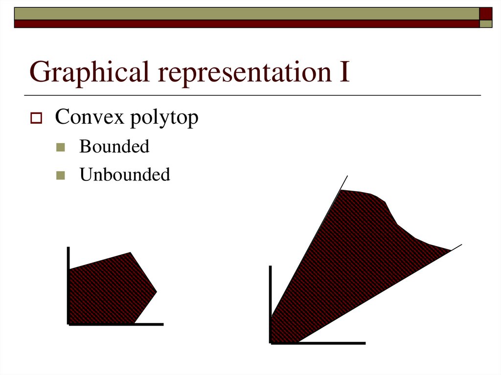
Graphical representation I
Convex polytop
Bounded
Unbounded

22.

Graphical representation II
Column space of matrix of coefficients
n
a x
j 1
j
j
b

23.

Simplex Method
Simplex method
Starts with a feasible solution
Tests whether or not it is optimum.
If not, the method proceeds a better solution
It is based on Jordanian elimination procedure.
It deals with equations and not with inequations

24.

The Simplex Algorithm
Step 0 – Initial simplex tableau
Step 1 – Test for optimality
STOP
Step 2 – Choose the entering variable
Step 3 – Test for unbounded objective function
Step 4 – Choose the leaving variable
Step 5 – Change the basis (JEM)
STOP

25.

The Simplex Algorithm
Converting LP into standard and canonical form
Definition of slack variables
Definition of artificial variables
Big M method
Equations, positive right hand side, canonical form
Test for optimality
zj is the amount of profit given by replacing some of the present basic
variables mix with one unit of the column variable
Determine the entering basic variable
Test for unbounded criterion and for feasibility
Determine the leaving basic variable
Changing basis
Jordanian elimination method

26.

Solubility of linear model
One optimal solution
Infinite number of optimal solution
Alternate solutions - If the zj - cj value for one or more
nonbasic variables is 0 in the optimal tableau,
No solution
Unbounded Linear programs
If all entries in the pivot column are nonpositive, the linear
program is unbounded.
Infeasible Linear Programs
If an artificial variable remains positive in the “optimal tableau,”
the problem is infeasible.

27.

Simple transportation problem
Suppliers, source – supply of i-th supplier ai
Demands, destinations – demand of j-th destination bj
Route (i,j) – unique connection between supplier and demand
Unit transportation costs (distances) between each origin
and destination – cij
xij – number of units shipped from supplier i to demand j
Goal: Minimize of the cost of shipping goods or maximize
the profit of shipping
27

28.

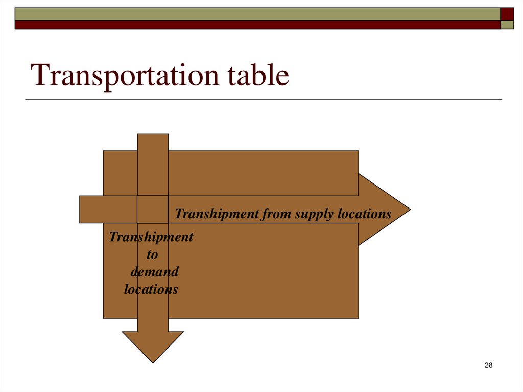
Transportation table
Transhipment from supply locations
Transhipment
to
demand
locations
28

29.

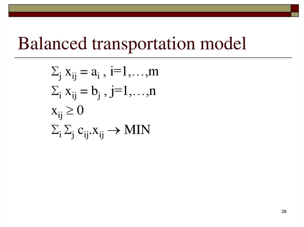
Balanced transportation model
j xij = ai , i=1,…,m
i xij = bj , j=1,…,n
xij 0
i j cij.xij MIN
29

30.

Balanced transportation system
Total supply = total demand j ai = j bj
dummy supplier
dummy destination
Frobenius theorem
If the system is balanced then the model is always solvable.
Basic solution m+n-1 basic variables (routes)
30

31.

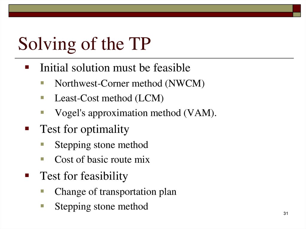
Solving of the TP
Initial solution must be feasible
Northwest-Corner method (NWCM)
Least-Cost method (LCM)
Vogel's approximation method (VAM).
Test for optimality
Stepping stone method
Cost of basic route mix
Test for feasibility
Change of transportation plan
Stepping stone method
31

32.

Transportation method
Step 0 – Balanced transportation system
Step 1 – Initial basic solution
Step 2 – Test for optimality
Step 3 – Test for feasibility
Step 4 – New basic solution

33.

Degeneracy
The basic solution is degenerate if some of basic
variables is equal to zero.
Degeneracy does not need some changes in the
simplex method.
Degeneracy requires to choose the missing basic
variable - to perform shipping stone method – in
transportation method.
(m + n – 1)
Degeneracy requires to choose the missing basic variable
so a closed path can be developed for all other empty
cells.

34.

Result analysis
Optimal solution
Alternative solution
Suboptimal solution
Perspective routes
Routes substitution
Possible shipped amount
34

35.

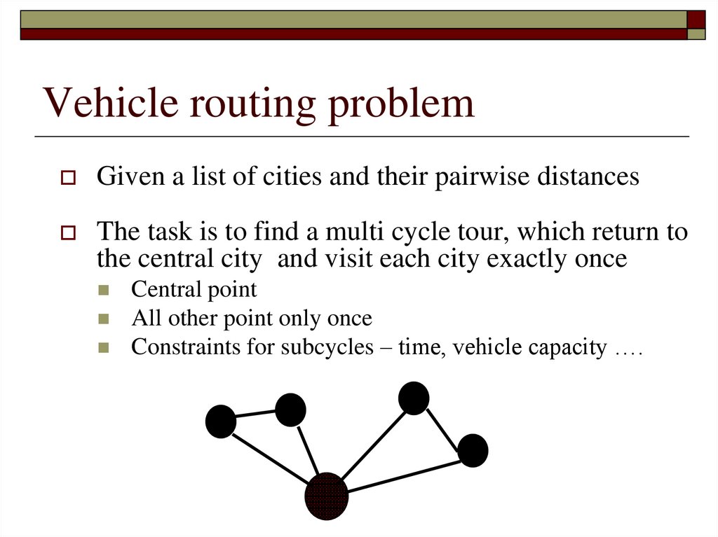
Vehicle routing problem
Given a list of cities and their pairwise distances
The task is to find a multi cycle tour, which return to
the central city and visit each city exactly once
Central point
All other point only once
Constraints for subcycles – time, vehicle capacity ….

36.

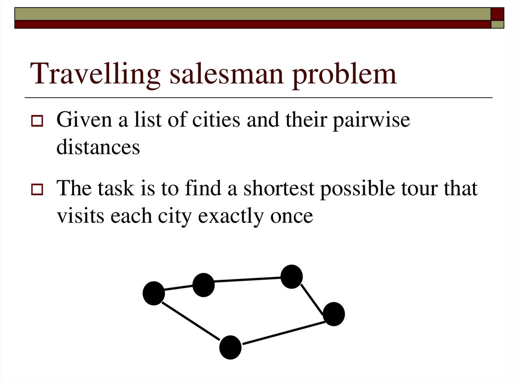
Travelling salesman problem
Given a list of cities and their pairwise
distances
The task is to find a shortest possible tour that
visits each city exactly once

37.

Solving of TSP
Try all permutations of points
N! possibilities
Principle: adding of branches to pass all points before
all points will be visited
Selection of branches according to the distance –
current advantage can be disadvantage in the future
The nearest neighbour algorithm
Vogel's Approximation Method

38.

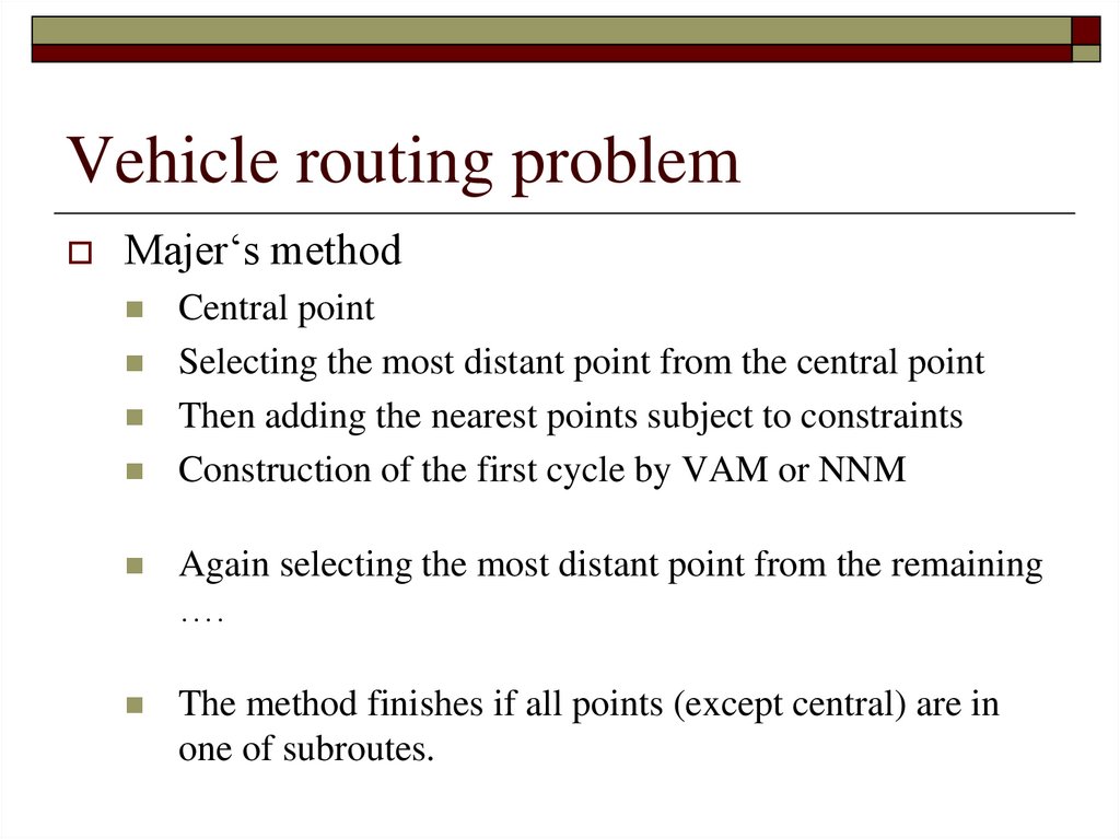
Vehicle routing problem
Majer‘s method
Central point
Selecting the most distant point from the central point
Then adding the nearest points subject to constraints
Construction of the first cycle by VAM or NNM
Again selecting the most distant point from the remaining
….
The method finishes if all points (except central) are in
one of subroutes.

39.

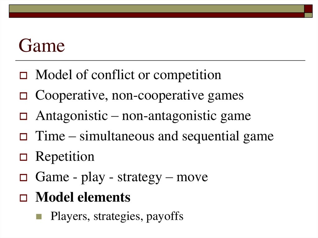
Game
Model of conflict or competition
Cooperative, non-cooperative games
Antagonistic – non-antagonistic game
Time – simultaneous and sequential game
Repetition
Game - play - strategy – move
Model elements
Players, strategies, payoffs

40.

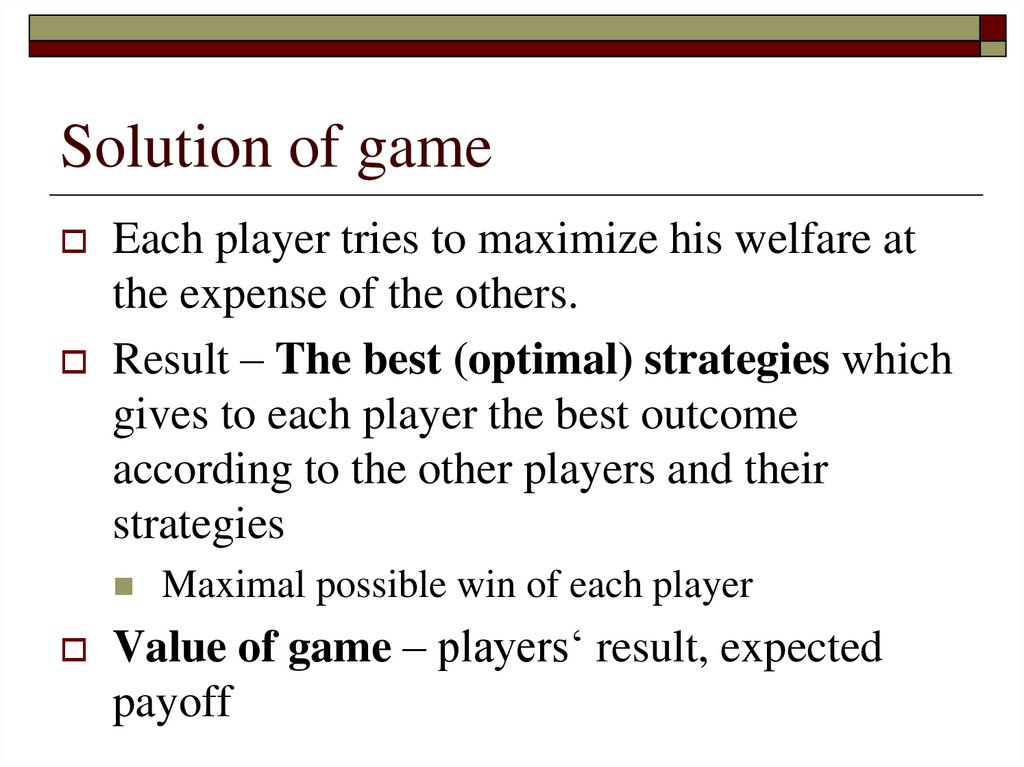
Solution of game
Each player tries to maximize his welfare at
the expense of the others.
Result – The best (optimal) strategies which
gives to each player the best outcome
according to the other players and their
strategies
Maximal possible win of each player
Value of game – players‘ result, expected
payoff

41.

Model of game
Tree (extensive) form of model
Game tree (decision tree - moves)
Normal form of model
List of players, list of strategy spaces, and list of
payoff functions
Payoff matrix (decision matrix)

42.

Matrix game
Two-person game
Finite number of strategies for each player
Zero-sum game
Sum of payoffs for both players is zero
Outcom of one player is a loss of the other player
Matrix form of game model

43.

Pure and mixed strategy
Pure strategy
One best strategy
How to find it – saddle point
Mixed strategy
Probability of strategy realization or frequency of
strategy usage
How to find it – linear optimization model

44.

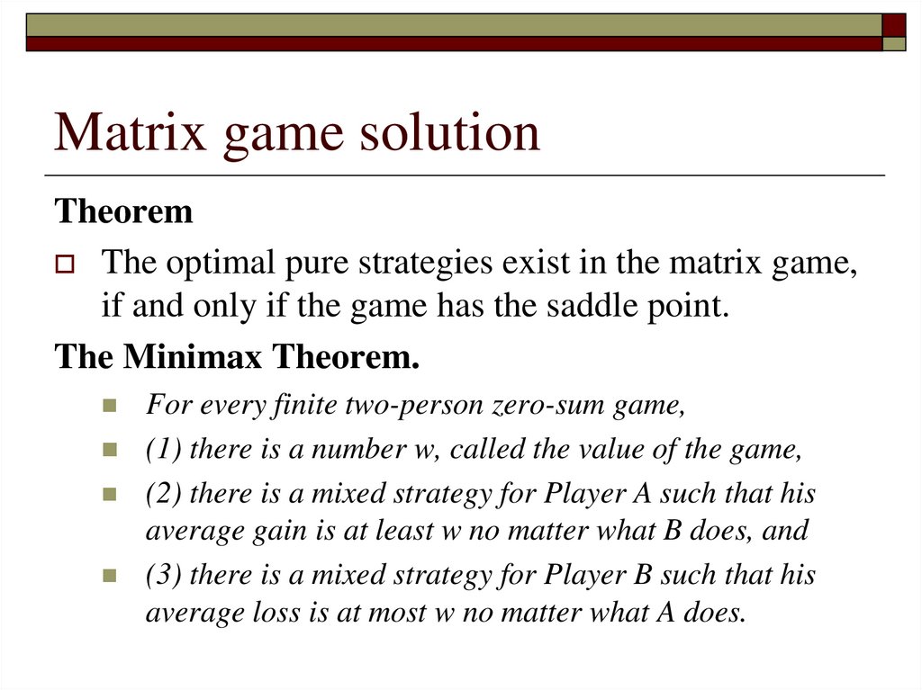
Matrix game solution
Theorem
The optimal pure strategies exist in the matrix game,
if and only if the game has the saddle point.
The Minimax Theorem.
For every finite two-person zero-sum game,
(1) there is a number w, called the value of the game,
(2) there is a mixed strategy for Player A such that his
average gain is at least w no matter what B does, and
(3) there is a mixed strategy for Player B such that his
average loss is at most w no matter what A does.

45.

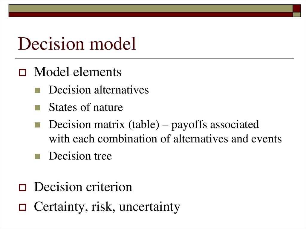
Decision model
Model elements
Decision alternatives
States of nature
Decision matrix (table) – payoffs associated
with each combination of alternatives and events
Decision tree
Decision criterion
Certainty, risk, uncertainty

46.

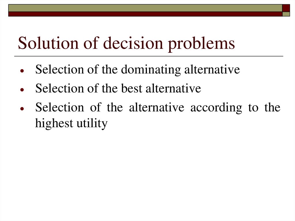
Solution of decision problems
Selection of the dominating alternative
Selection of the best alternative
Selection of the alternative according to the
highest utility

47.

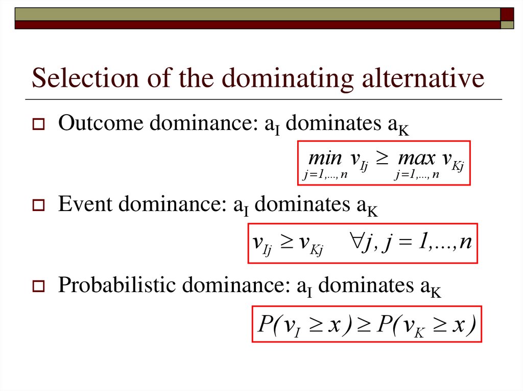
Selection of the dominating alternative
Outcome dominance: aI dominates aK
min vIj max vKj
j 1,..., n
Event dominance: aI dominates aK
vIj vKj
j 1,..., n
j , j 1,...,n
Probabilistic dominance: aI dominates aK
P( vI x ) P( vK x )

48.

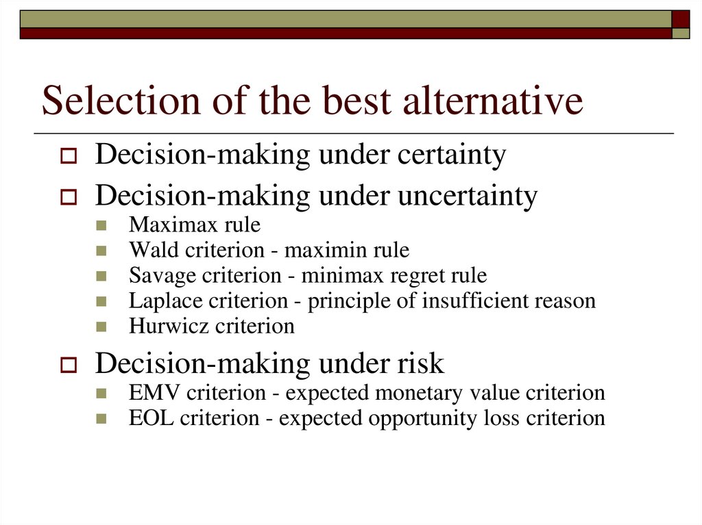
Selection of the best alternative
Decision-making under certainty
Decision-making under uncertainty
Maximax rule
Wald criterion - maximin rule
Savage criterion - minimax regret rule
Laplace criterion - principle of insufficient reason
Hurwicz criterion
Decision-making under risk
EMV criterion - expected monetary value criterion
EOL criterion - expected opportunity loss criterion

49.

Multiple Objective Decision Making
Infinite Number of Alternatives
At least two criteria
Example – Linear multi criteria programming
y1 ( x) c x MAX
T
yk ( x) ck x MIN
Ax b
x 0
T
1

50.

Multiple Attribute Decision Making
Finite Number of Alternatives
Evaluation of all alternatives with respect to
all attributes
f1
a1
a2
ap
y11
y21
y
p1
f2
y12
y22
yp2
fk
y1k
y2 k
y pk

51.

Basic terms
Ideal alternative
Nadir alternative
Dominating and dominated alternative
The best alternative – preferred alternative
Pareto efficient alternative

52.

The aim of MADM
Selection of the best alternatives (one or more)
Dichotomizing into the efficient and non
efficient alternatives
Ranking of all alternatives
Noncompensatory model
Not permit trade-offs between attributes
Compensatory Model
Permit trade-offs between attributes

53.

Utility, utility function
Utility is a measure of satisfaction
All attribute values can be expresed by utility
value
Partial utility values can be combined into
global utility value
Risk seeking, risk neutral and risk aversion
decision maker

54.

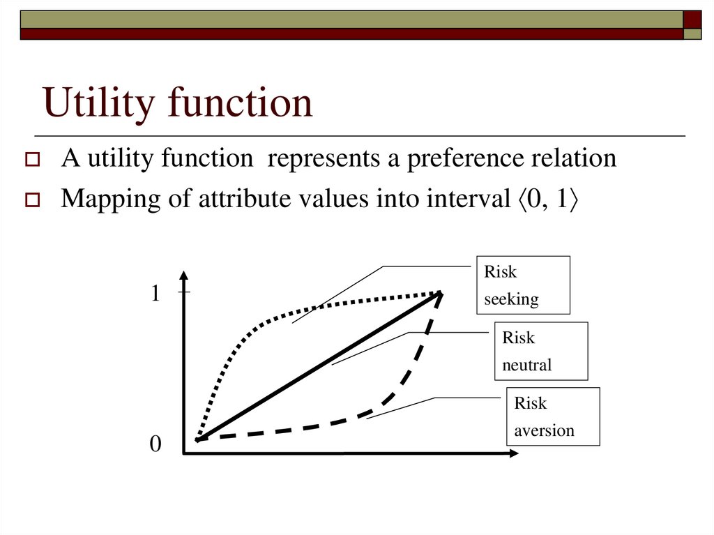
Utility function
A utility function represents a preference relation
Mapping of attribute values into interval 0, 1
Risk
1
seeking
Risk
neutral
Risk
0
aversion

55.

Informations
Inter and intra attribute comparisons
Criteria preferences
Alternatives preferences
Not necessary in numerical form
No preference information given
Nominal information – standard level of attribute
Ordinal information – qualitative - ordering
Cardinal information - quantitative

56.

Methods for assesing information
Sequence Method
Scoring Method
Criteria/alternatives are arranged according their importance
to a sequence from most to least important.
Each criterion/alternative isevaluated by certain number of
points from chosen scale.
Pairwise comparison
The judgement of the relative importance of each pair of
criteria

57.

MADM methods
Scoring or sequence methods
Standard level methods
Simple additive weighting method
Attributes must be measured in the same scale

58.

Credit and Exam
Credit specifications
Selftests in Moodle – 60 % of points
Resit credit test – 60 % of points
Exam specifications
Exam written test – 60 % of points
Theory – 2 questions (15 points each)
Small example (30 points)
Practical application (40 points)
Oral examination (immediately after test)