The linear programming. (Lecture 5)

1.

National Aviation University
Department of Airnavigation system
Lecture 5: The Linear Programming
1.
2.
3.
4.
What Is Operations Research? (OR)
The Linear Programming tasks
Tasks: Computers Purchase and Diet Problem
Determine the Linear Programming tasks using MS Excel
Professor Shmelova T.

2.

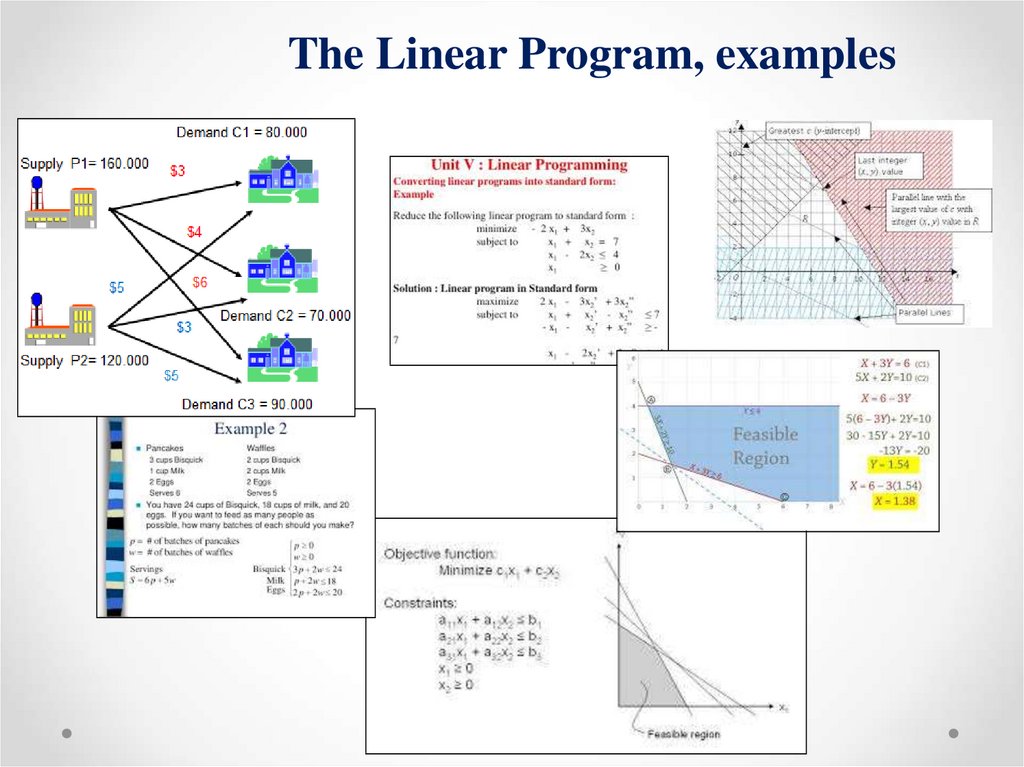
The Linear Program, examples

3.

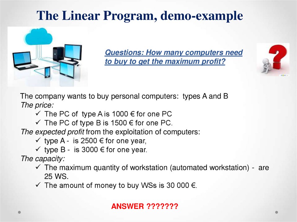
The Linear Program, demo-example
Questions: How many computers need
to buy to get the maximum profit?
The company wants to buy personal computers: types A and B
The price:
The PC of type A is 1000 € for one PC
The PC of type B is 1500 € for one PC.
The expected profit from the exploitation of computers:
type A - is 2500 € for one year,
type B - is 3000 € for one year.
The capacity:
The maximum quantity of workstation (automated workstation) - are
25 WS.
The amount of money to buy WSs is 30 000 €.
ANSWER ???????

4.

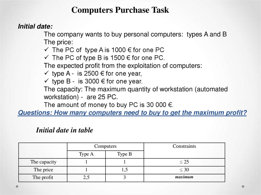
Computers Purchase Task
Initial date:
The company wants to buy personal computers: types A and B
The price:
The PC of type A is 1000 € for one PC
The PC of type B is 1500 € for one PC.
The expected profit from the exploitation of computers:
type A - is 2500 € for one year,
type B - is 3000 € for one year.
The capacity: The maximum quantity of workstation (automated
workstation) - are 25 PC.
The amount of money to buy PC is 30 000 €.
Questions: How many computers need to buy to get the maximum profit?
Initial date in table
Computers
Constraints
Type A
Type B
The capacity
1
1
25
The price
1
1,5
30
The profit
2,5
3
maximum

5.

Computers
Constraints
Type A
Type B
The capacity
1
1
25
The price
1
1,5
30
The profit
2,5
3
maximum

6.

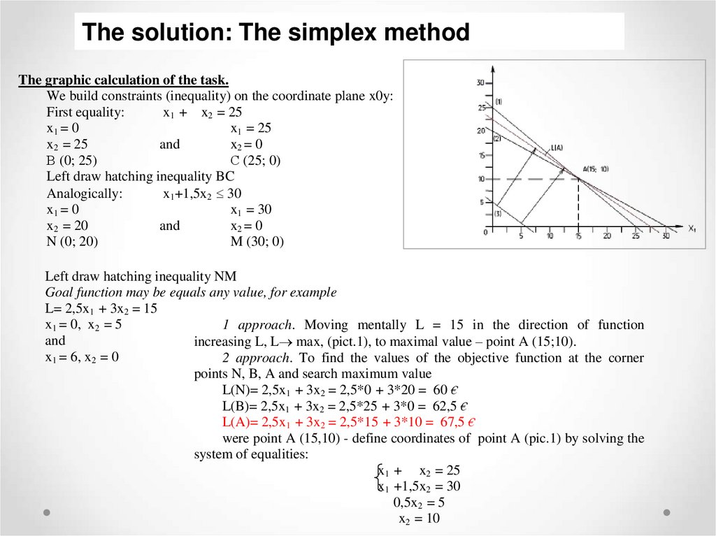
The solution: The simplex method
The graphic calculation of the task.
We build constraints (inequality) on the coordinate plane x0y:
First equality:
x1 + x2 = 25
x1 = 0
x1 = 25
x2 = 25
and
x2 = 0
В (0; 25)
С (25; 0)
Left draw hatching inequality BC
Analogically:
x1+1,5x2 30
x1 = 0
x1 = 30
x2 = 20
and
x2 = 0
N (0; 20)
M (30; 0)
Left draw hatching inequality NM
Goal function may be equals any value, for example
L= 2,5x1 + 3x2 = 15
x1 = 0, x2 = 5
1 approach. Moving mentally L = 15 in the direction of function
and
increasing L, L max, (pict.1), to maximal value – point A (15;10).
x1 = 6, x2 = 0
2 approach. To find the values of the objective function at the corner
points N, B, A and search maximum value
L(N)= 2,5x1 + 3x2 = 2,5*0 + 3*20 = 60 €
L(B)= 2,5x1 + 3x2 = 2,5*25 + 3*0 = 62,5 €
L(A)= 2,5x1 + 3x2 = 2,5*15 + 3*10 = 67,5 €
were point A (15,10) - define coordinates of point A (pic.1) by solving the
system of equalities:
x1 + x2 = 25
x1 +1,5x2 = 30
0,5x2 = 5
x2 = 10

7.

ANSWER :
Maximum value of in point A of the objective function:
L(A) = 67,5
Optimal solution:
x1 = 15 – PC of type A
x2 = 10 – PC of type B
Сheck:
The amount of money to buy PC is 30 000 €:
1000*15+1500*10 = 30000
The capacity - quantity of workstation:
15 + 10 = 25 PC
THE RESULT: The optimal quantity of computers type A that used to be
bought is 15, type B is 10 computers. At the same time the maximal
profit of both types computer’s exploitation will be 67,5 €

8.

1. What Is Operations Research? (OR)
The first formal activities of Operations Research (OR) were
initiated in England, USA, USSR, other countries during World
War II, when scientists set out to make scientifically based
decisions regarding the best utilization of war materiel.
After the war, the ideas advanced in military operations were
adapted to improve efficiency and productivity in the civilian
sector.
Operations research, or operational research, is a
discipline that deals with the application of advanced analytical
methods to help make better decisions.
Mathematical model of linear program (LP) tasks:
The simplex method – main method of decisions LP tasks

9.

General phases (stages) of construction of a mathematical
model (OR):
The principal phases for implementing OR in practice include:
1. Definition of the problem (alternatives, feasible variables, constrains, goal,..)
2. Construction of the model.
3. Solution of the task.
4. Validation of the model.
5. Implementation of the solution in practice.
The LP mathematical model, as in any OR model, has three stages of construction:
1.To find the variables x1, x2, x3, …
2.To find constraints
3.To find an objective function (goal) that we need to optimize (maximum or
minimum) – L

10.

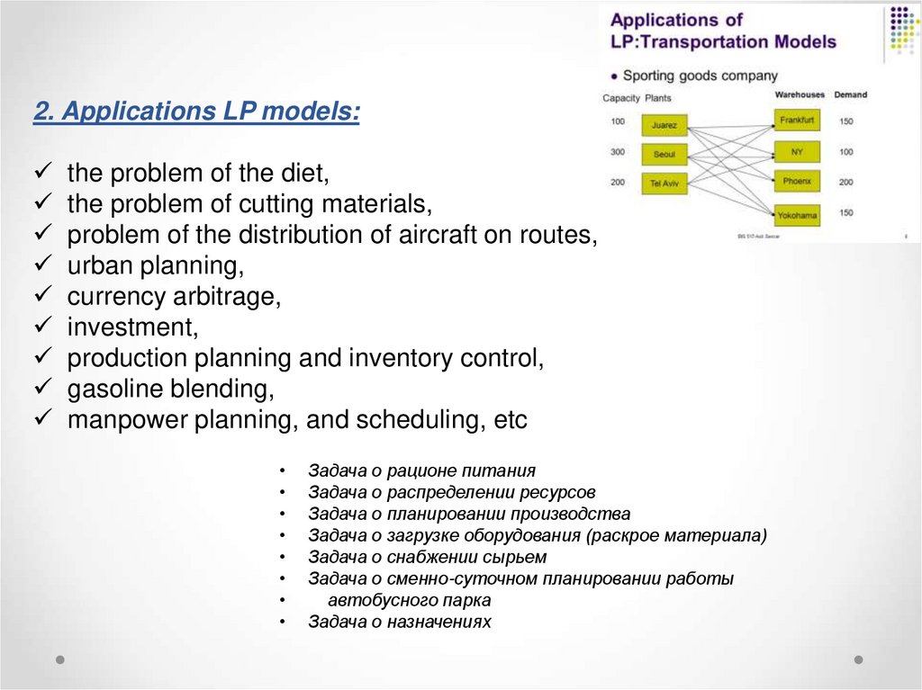
2. Applications LP models:
the problem of the diet,
the problem of cutting materials,
problem of the distribution of aircraft on routes,
urban planning,
currency arbitrage,
investment,
production planning and inventory control,
gasoline blending,
manpower planning, and scheduling, etc
Задача о рационе питания
Задача о распределении ресурсов
Задача о планировании производства
Задача о загрузке оборудования (раскрое материала)
Задача о снабжении сырьем
Задача о сменно-суточном планировании работы
автобусного парка
Задача о назначениях

11.

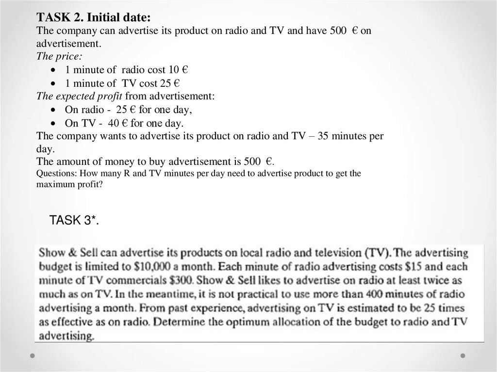
TASK 2. Initial date:
The company can advertise its product on radio and TV and have 500 € on
advertisement.
The price:
1 minute of radio cost 10 €
1 minute of TV cost 25 €
The expected profit from advertisement:
On radio - 25 € for one day,
On TV - 40 € for one day.
The company wants to advertise its product on radio and TV – 35 minutes per
day.
The amount of money to buy advertisement is 500 €.
Questions: How many R and TV minutes per day need to advertise product to get the
maximum profit?
TASK 3*.

12.

Determine the Linear Programming tasks using MS Excel
Main steps
1.Make the task form
2.Enter basic data of the task to the form:
Enter the dependence for the criterion function (”Function Master” fx ;
“СУММПРОИЗВ” (category: mathematical))
Enter the dependence for the left part of constrains
3. Working in dialogue box Solution search:
Enter the direction of criterion function
Inscribe the constrains in area "The limitation"
4. The shunt in " Characteristic "

13.

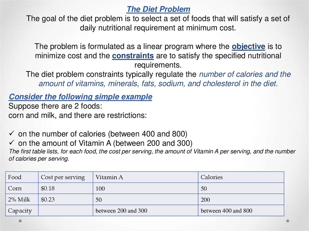
The Diet Problem
The goal of the diet problem is to select a set of foods that will satisfy a set of
daily nutritional requirement at minimum cost.
The problem is formulated as a linear program where the objective is to
minimize cost and the constraints are to satisfy the specified nutritional
requirements.
The diet problem constraints typically regulate the number of calories and the
amount of vitamins, minerals, fats, sodium, and cholesterol in the diet.
Consider the following simple example
Suppose there are 2 foods:
corn and milk, and there are restrictions:
on the number of calories (between 400 and 800)
on the amount of Vitamin A (between 200 and 300)
The first table lists, for each food, the cost per serving, the amount of Vitamin A per serving, and the number
of calories per serving.
Food
Cost per serving
Vitamin A
Calories
Corn
$0.18
100
50
2% Milk
$0.23
50
200
between 200 and 300
between 400 and 800
Capacity

14.

The LP model, as in any OR model, has three basic components.
1. Decision variables that we seek to determine:
xi - number of servings of food i to purchase/consume
x1 - Corn
x2 - 2% Milk
2. Constraints that the solution must satisfy:
- the capacity of Vitamin A:
100x1 +50 x2 300
100x1 +50 x2 ≥ 200
-the capacity of Calories:
50x1+200x2 800
50x1+200x2 ≥ 400
3. Objective (goal) that we need to optimize (maximize or minimize).
Secondly the cost of food should be minimum:
F = 0,18x1+0,23x2 min

15.

Solution
Mathematical model:
Objective
F = 0,18x1+0,23x2 min
restrictions:
107x1 +500 x2 50000
107x1 +500 x2 ≥ 5000
72x1+121x2 2250
72x1+121x2 ≥ 2000
x1 0
x2 0
x1
1
100x1 +50 x2 300
2
100x1 +50 x2 ≥ 200
3
50x1+200x2 800
4
50x1+200x2 ≥ 400
x2
0
3
0
2
0
16
0
8
6
0
4
0
4
0
2
0
4
8
1,7
1,8
0,92
2,074
0,841
0,594
x1 ³ 0
x2 ³ 0
F = 0,18x1+0,23x2
A(0;4)
B(1;3,8)
C(2,5;1,7)
D(1;1,8)
0
1,3
2,50
1
0; 6
3; 0
0; 4
2; 0
0; 4
16; 0
0; 2
8; 0

16.

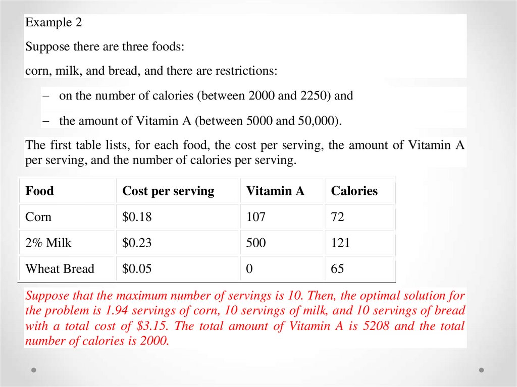
Example 2
Suppose there are three foods:
corn, milk, and bread, and there are restrictions:
on the number of calories (between 2000 and 2250) and
the amount of Vitamin A (between 5000 and 50,000).
The first table lists, for each food, the cost per serving, the amount of Vitamin A
per serving, and the number of calories per serving.
Food
Cost per serving
Vitamin A
Calories
Corn
$0.18
107
72
2% Milk
$0.23
500
121
Wheat Bread
$0.05
0
65
Suppose that the maximum number of servings is 10. Then, the optimal solution for
the problem is 1.94 servings of corn, 10 servings of milk, and 10 servings of bread
with a total cost of $3.15. The total amount of Vitamin A is 5208 and the total
number of calories is 2000.

17.

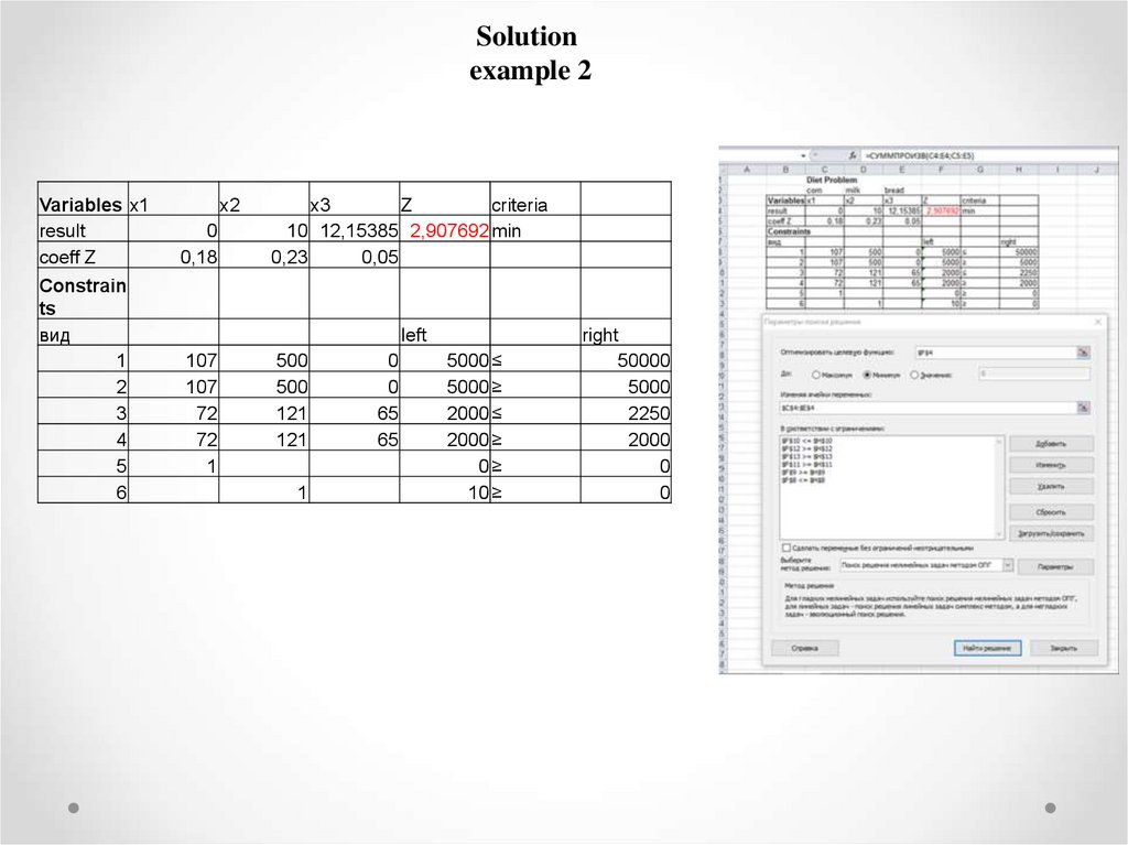
Solution
example 2
Variables x1
result
coeff Z
Constrain
ts
вид
1
2
3
4
5
6
x2
0
0,18
x3
Z
criteria
10 12,15385 2,907692 min
0,23
0,05
left
107
107
72
72
1
500
500
121
121
1
0
0
65
65
5000 ≤
5000 ≥
2000 ≤
2000 ≥
0≥
10 ≥
right
50000
5000
2250
2000
0
0

18.

4. Determine the Linear Programming tasks using MS Excel
Operation algorithm for the sum solving:
Make the task form (pic.2.5).
Enter basic data of the task /2.3/ - /2.4/ to the form(pic.2.6).
Enter the dependence from the mathematical simulator /2.3/ - /2.4/ to
1.
2.
3.
the form:
3.1. Enter the dependence for the criterion function /2.3/:
The shunt to the cell F6
The shunt to the button”Function Master” fx
At the screen: dialogue box " Function Master–step1 from 2"
The shunt to the function box “СУММПРОИЗВ” (category
:mathematical)
“OK”
At the screen: dialogue box “СУММПРОИЗВ”
In array1 enter В3:C3 (allocate by mouse )
In array 2 enter В6:C6
"ОК"
At the screen: in F6 was entered criterion function data
“=СУММПРОИЗВ(В3:C3;В6:C6)”

19.

3.2.Enter the dependence for the left part of limitations:
The shunt to the cell F9
The shunt to the button”Function Master” fx
At the screen: dialogue box " Function Master–step1 from 2"
The shunt to the function box “СУММПРОИЗВ”
“OK”
At the screen: dialogue box “СУММПРОИЗВ”
In array1 enter В3:C3 (allocate by mouse)
In array 2 enter В9:C9
"ОК"
(the same way for the F10)
At the screen:
In F9 “=СУММПРОИЗВ(В3:C3;В9:C9)”;
in F10 “=СУММПРОИЗВ(В3:C3;В10:C10)”.
Basic data entering is over.

20.

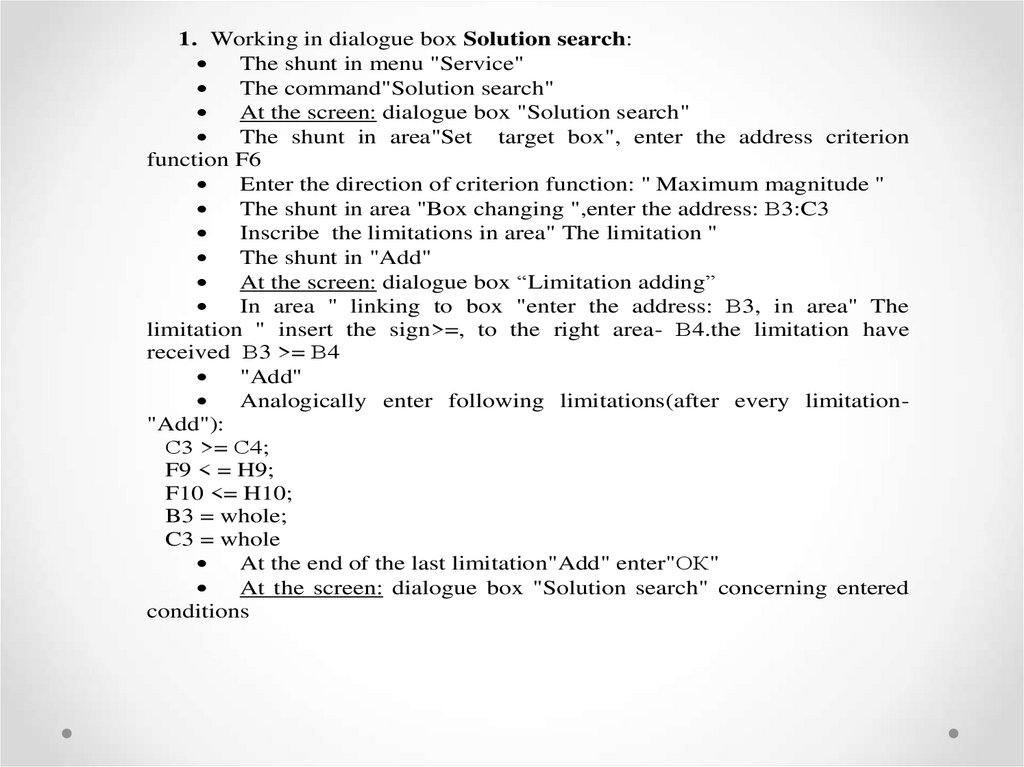
1. Working in dialogue box Solution search:
The shunt in menu "Service"
The command"Solution search"
At the screen: dialogue box "Solution search"
The shunt in area"Set target box", enter the address criterion
function F6
Enter the direction of criterion function: " Maximum magnitude "
The shunt in area "Box changing ",enter the address: В3:C3
Inscribe the limitations in area" The limitation "
The shunt in "Add"
At the screen: dialogue box “Limitation adding”
In area " linking to box "enter the address: В3, in area" The
limitation " insert the sign>=, to the right area- В4.the limitation have
received В3 >= В4
"Add"
Analogically enter following limitations(after every limitation"Add"):
С3 >= С4;
F9 < = H9;
F10 <= H10;
B3 = whole;
C3 = whole
At the end of the last limitation"Add" enter"ОК"
At the screen: dialogue box "Solution search" concerning entered
conditions

21.

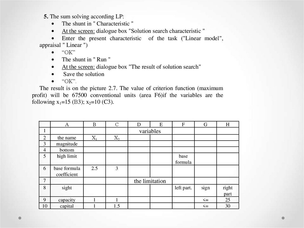
5. The sum solving according LP:
The shunt in " Characteristic "
At the screen: dialogue box "Solution search characteristic "
Enter the present characteristic of the task ("Linear model",
appraisal " Linear ")
“ОК”
The shunt in " Run "
At the screen: dialogue box "The result of solution search"
Save the solution
“ОК”.
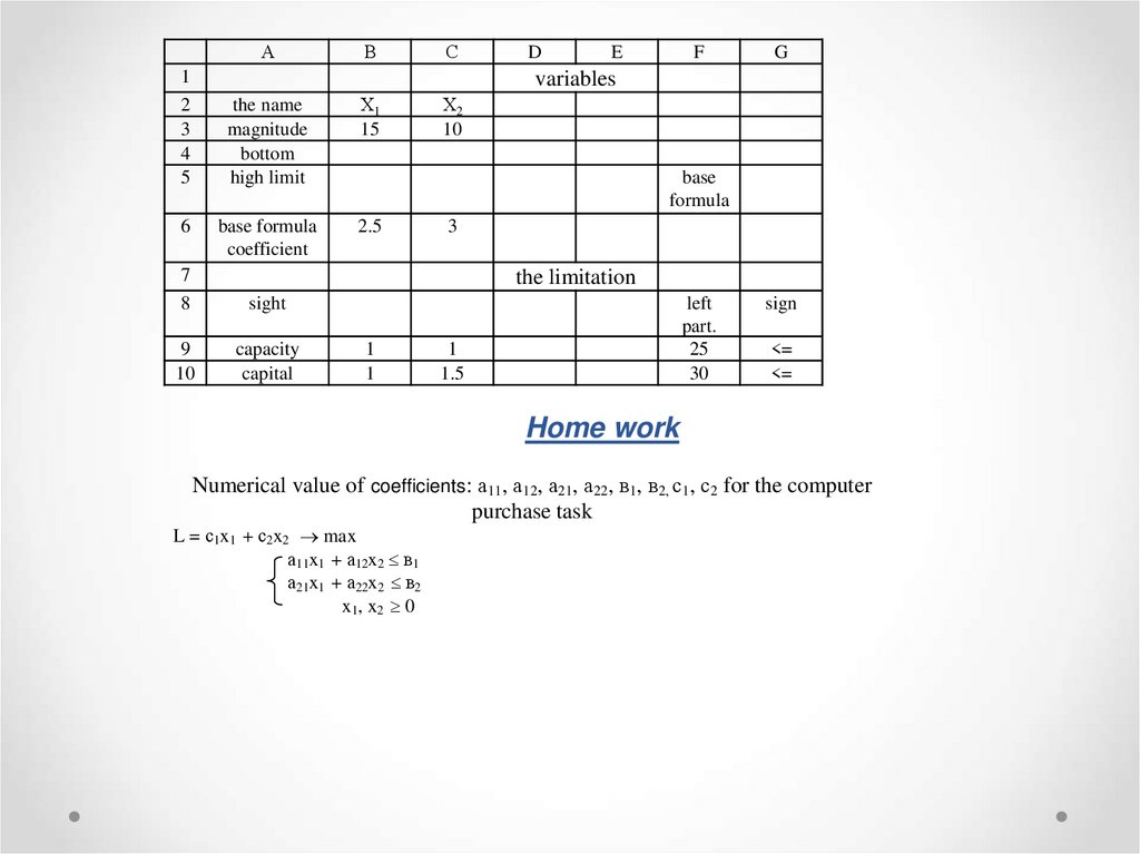
The result is on the picture 2.7. The value of criterion function (maximum
profit) will be 67500 conventional units (area F6)if the variables are the
following x1=15 (В3); x2=10 (C3).
А
1
2
3
4
5
6
В
С
D
E
F
G
H
sign
right
part
25
30
variables
the name
magnitude
bottom
high limit
Х1
base formula
coefficient
2.5
7
8
sight
9
10
capacity
capital
Х2
base
formula
3
the limitation
left part.
1
1
1
1.5
<=
<=

22.

А
1
2
3
4
5
В
С
D
E
F
G
variables
6
the name
magnitude
bottom
high limit
Х1
15
base formula
coefficient
2.5
7
8
sight
9
10
capacity
capital
Х2
10
base
formula
3
the limitation
1
1
left
part.
25
30
1
1.5
sign
<=
<=
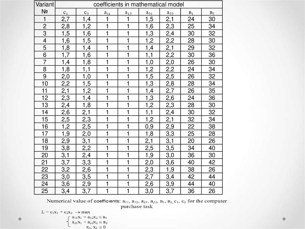
Home work
Numerical value of coefficients: а11, а12, а21, а22, в1, в2, с1, с2 for the computer
purchase task
L = с1x1 + с2x2 max
а11x1 + а12x2 в1
а21x1 + а22x2 в2
x1 , x 2 0

23.

Variant
№
1
2
3
4
5
6
7
8
9
10
11
12
13
14
15
16
17
18
19
20
21
22
23
24
25
с1
2,7
2,8
1,5
1,6
1,8
1,7
1,4
1,8
2,0
2,2
2,1
2,3
2,4
2,6
2,5
1,2
1,9
2,9
3,8
3,1
3,7
3,2
3,0
3,6
3,4
с2
1,4
1,2
1,6
1,5
1,4
1,6
1,8
1,1
1,0
1,5
1,2
1,4
1,8
2,1
2,3
2,5
2,0
3,1
2,2
2,4
3,3
2,6
3,5
2,9
3,7
coefficients in mathematical model
а11
а12
а21
а22
1
1
1,5
2,1
1
1
1,6
2,3
1
1
1,3
2,4
1
1
1,2
2,2
1
1
1,4
2,1
1
1
1,1
2,2
1
1
1,0
2,0
1
1
1,2
2,2
1
1
1,5
2,5
1
1
1,3
2,8
1
1
1,4
2,7
1
1
1,3
2,6
1
1
1,2
2,3
1
1
1,1
2,4
1
1
1,2
2,1
1
1
0,9
2,9
1
1
1,8
3,3
1
1
2,1
3,1
1
1
2,5
3,5
1
1
1,9
3,0
1
1
2,0
3,6
1
1
2,3
1,9
1
1
2,7
3,4
1
1
2,6
3,9
1
1
3,0
3,7
в1
24
25
30
28
29
30
26
24
26
28
26
24
28
30
32
22
25
20
34
36
40
38
42
44
36
в2
30
34
32
30
32
36
30
34
32
34
35
36
30
32
34
38
28
26
40
30
42
26
44
40
26

24. Thank you for your attention