Эволюционные модели и дистанции между последовательностями биополимеров

1.

Эволюционные модели и дистанции
между последовательностями
биополимеров
Молекулярная филогения
Статистические методы оценки деревьев.
Анализ молекулярных часов.

2.

3.

4.

5.

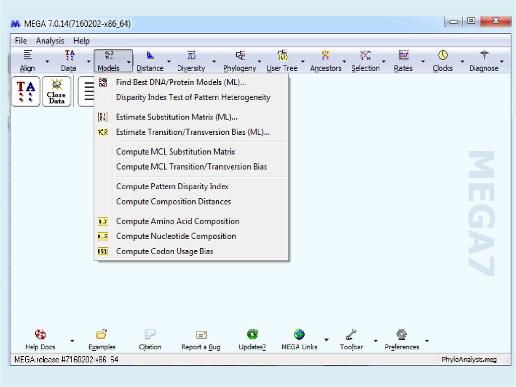
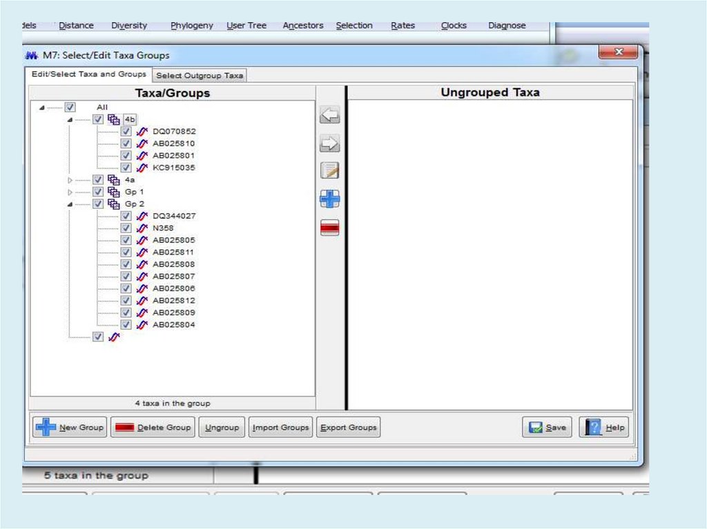
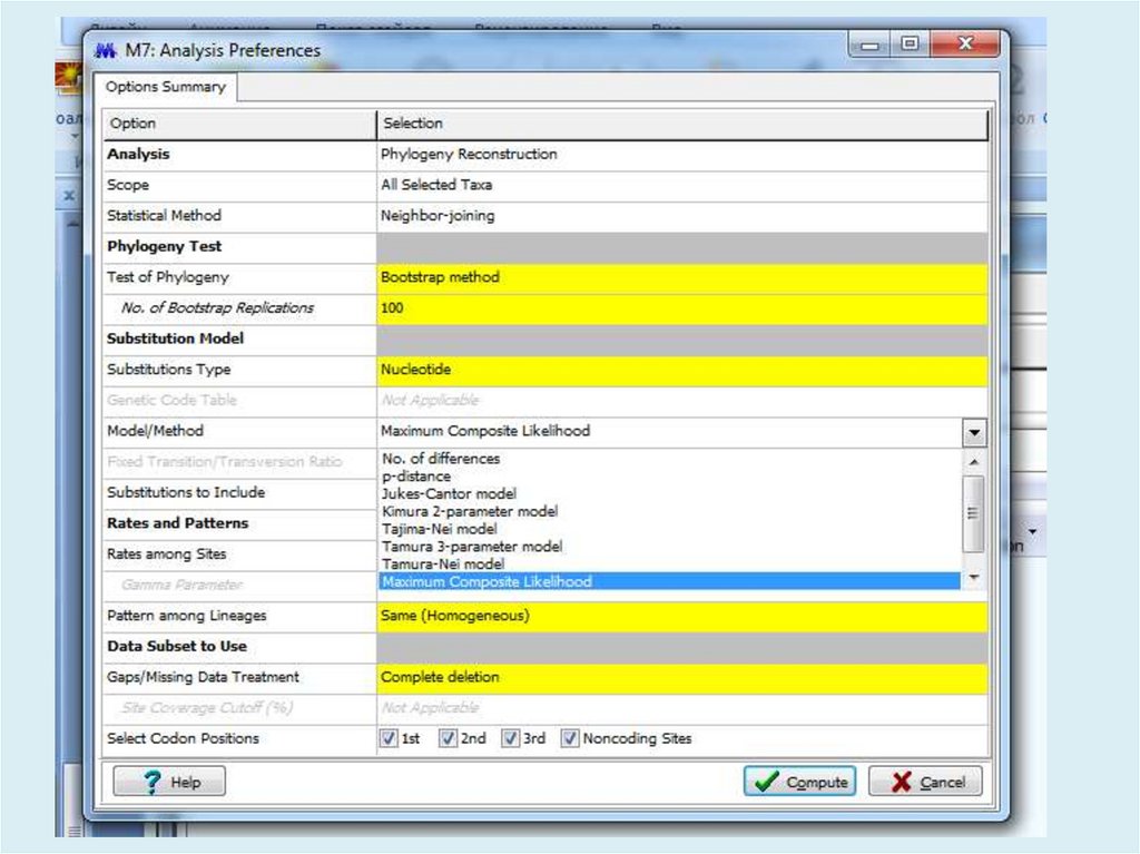
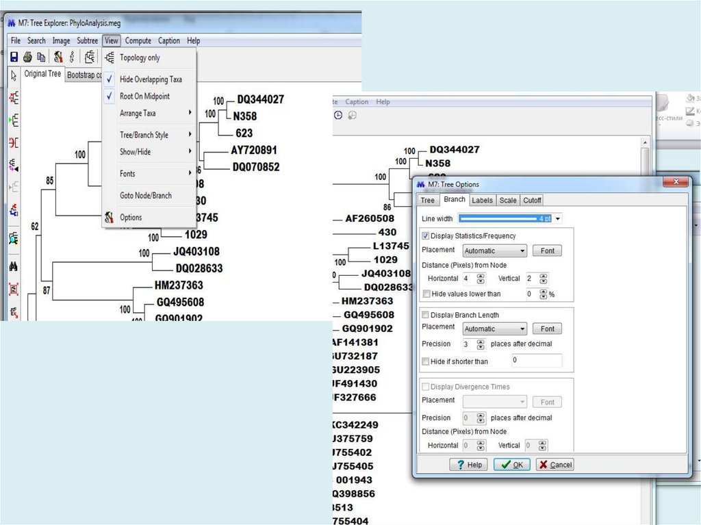
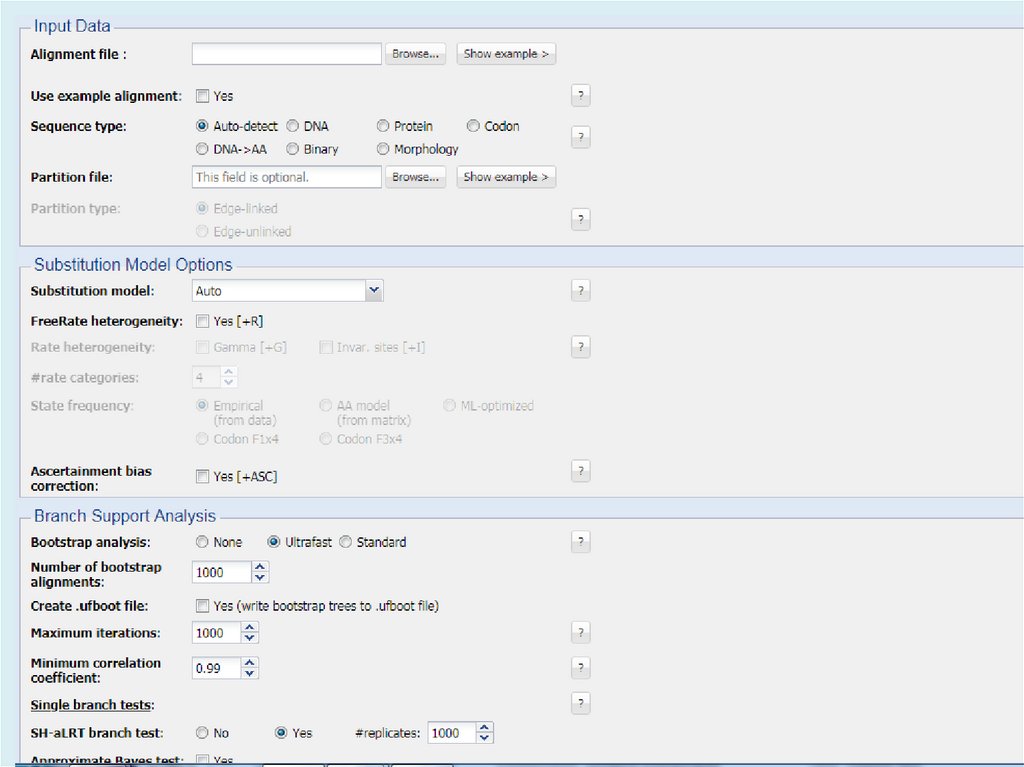
Для анализа с использованием метода максимального правдоподобия, параметр
«branch swap filter» используется для установки строгости оптимизации
относительно длины ветви. Более слабый фильтр приведет к более исчерпывающей
оптимизации, однако поиск может занять больше времени, но потенциально,
большее пространство будет изучено.

6.

7.

8.

9.

10.

11.

12.

13.

14.

15.

16.

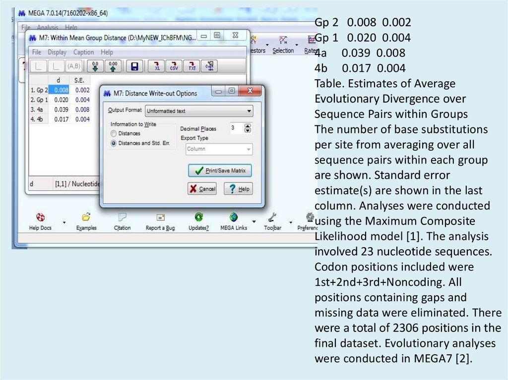
Gp 2 0.008 0.002
Gp 1 0.020 0.004
4a 0.039 0.008
4b 0.017 0.004
Table. Estimates of Average
Evolutionary Divergence over
Sequence Pairs within Groups
The number of base substitutions
per site from averaging over all
sequence pairs within each group
are shown. Standard error
estimate(s) are shown in the last
column. Analyses were conducted
using the Maximum Composite
Likelihood model [1]. The analysis
involved 23 nucleotide sequences.
Codon positions included were
1st+2nd+3rd+Noncoding. All
positions containing gaps and
missing data were eliminated. There
were a total of 2306 positions in the
final dataset. Evolutionary analyses
were conducted in MEGA7 [2].

17.

[1]
[2]
[3]
[4]
[
[1]
[2]
[3]
[4]
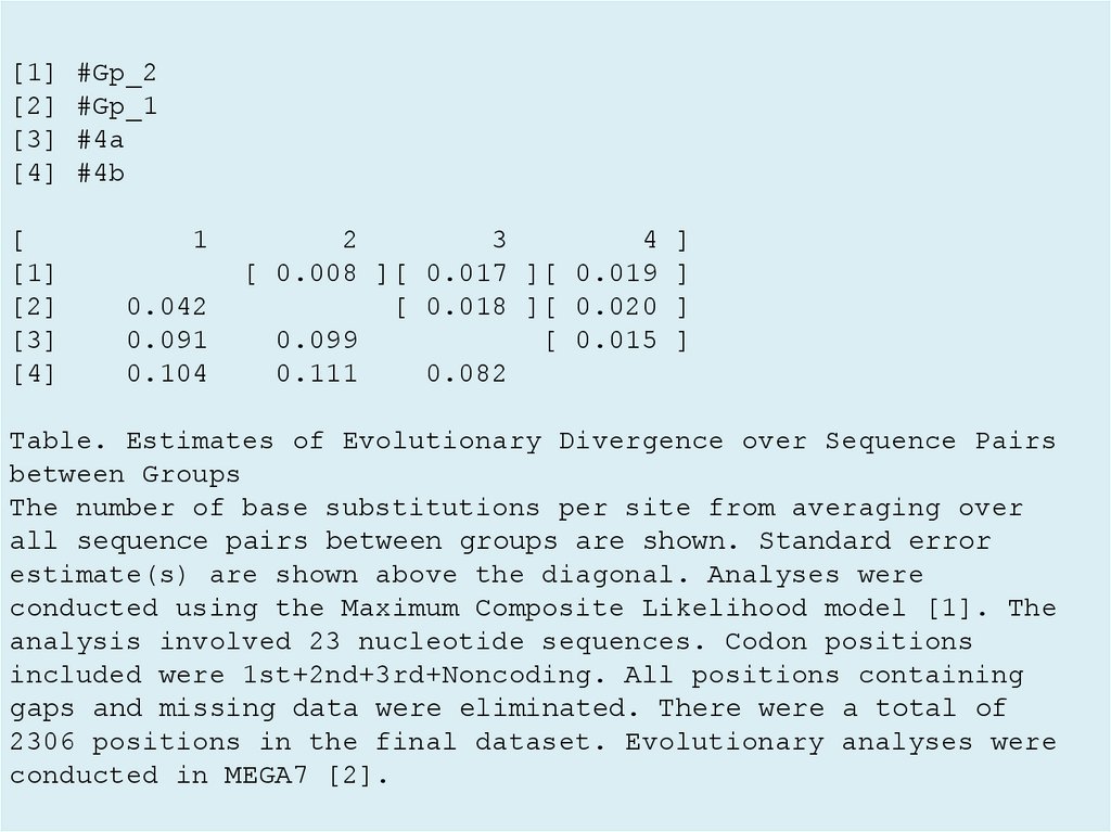
#Gp_2
#Gp_1
#4a
#4b
1
0.042
0.091
0.104
2
3
4
[ 0.008 ][ 0.017 ][ 0.019
[ 0.018 ][ 0.020
0.099
[ 0.015
0.111
0.082
]
]
]
]
Table. Estimates of Evolutionary Divergence over Sequence Pairs
between Groups
The number of base substitutions per site from averaging over
all sequence pairs between groups are shown. Standard error
estimate(s) are shown above the diagonal. Analyses were
conducted using the Maximum Composite Likelihood model [1]. The
analysis involved 23 nucleotide sequences. Codon positions
included were 1st+2nd+3rd+Noncoding. All positions containing
gaps and missing data were eliminated. There were a total of
2306 positions in the final dataset. Evolutionary analyses were
conducted in MEGA7 [2].

18.

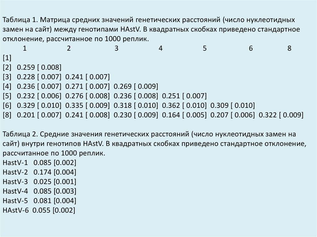
Таблица 1. Матрица средних значений генетических расстояний (число нуклеотидных
замен на сайт) между генотипами HAstV. В квадратных скобках приведено стандартное
отклонение, рассчитанное по 1000 реплик.
1
2
3
4
5
6
8
[1]
[2] 0.259 [ 0.008]
[3] 0.228 [ 0.007] 0.241 [ 0.007]
[4] 0.236 [ 0.007] 0.271 [ 0.007] 0.269 [ 0.009]
[5] 0.232 [ 0.006] 0.276 [ 0.008] 0.236 [ 0.008] 0.251 [ 0.007]
[6] 0.329 [ 0.010] 0.335 [ 0.009] 0.318 [ 0.010] 0.362 [ 0.010] 0.309 [ 0.010]
[8] 0.201 [ 0.007] 0.241 [ 0.008] 0.230 [ 0.009] 0.164 [ 0.005] 0.207 [ 0.006] 0.322 [ 0.009]
Таблица 2. Средние значения генетических расстояний (число нуклеотидных замен на
сайт) внутри генотипов HAstV. В квадратных скобках приведено стандартное отклонение,
рассчитанное по 1000 реплик.
HastV-1 0.085 [0.002]
HastV-2 0.174 [0.004]
HastV-3 0.025 [0.001]
HastV-4 0.085 [0.003]
HastV-5 0.081 [0.004]
HAstV-6 0.055 [0.002]

19.

20.

21.

22.

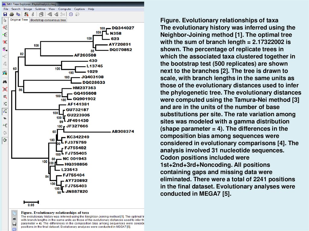
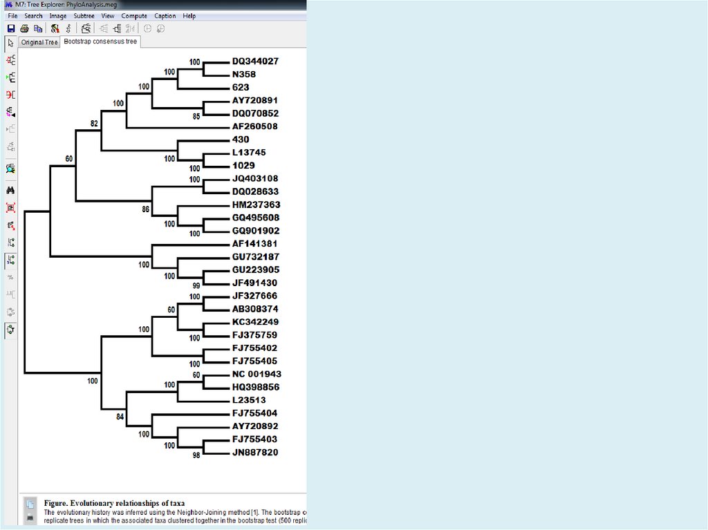
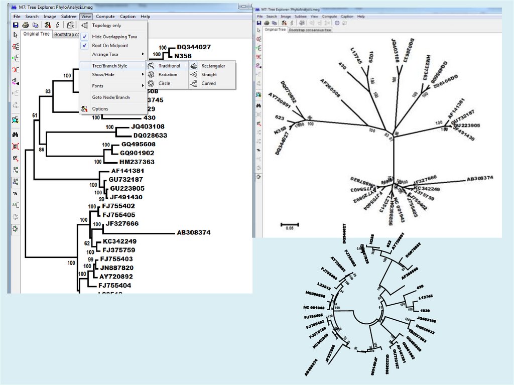
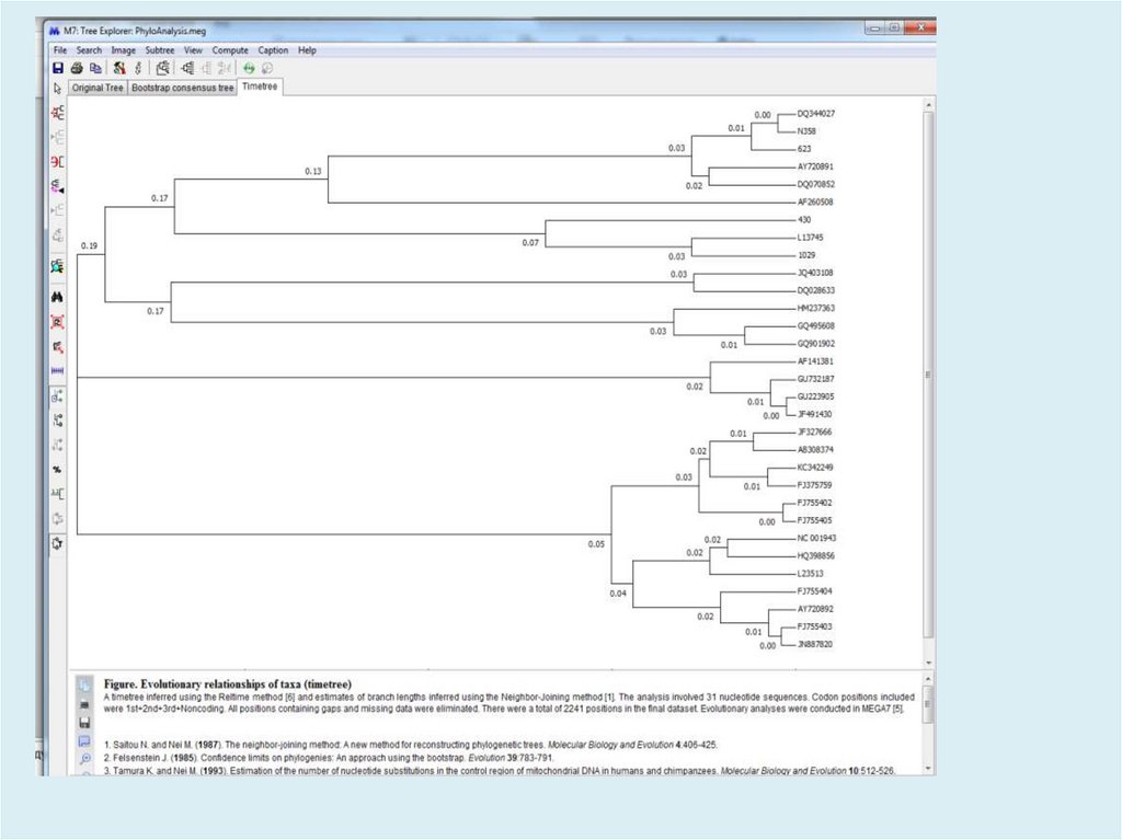
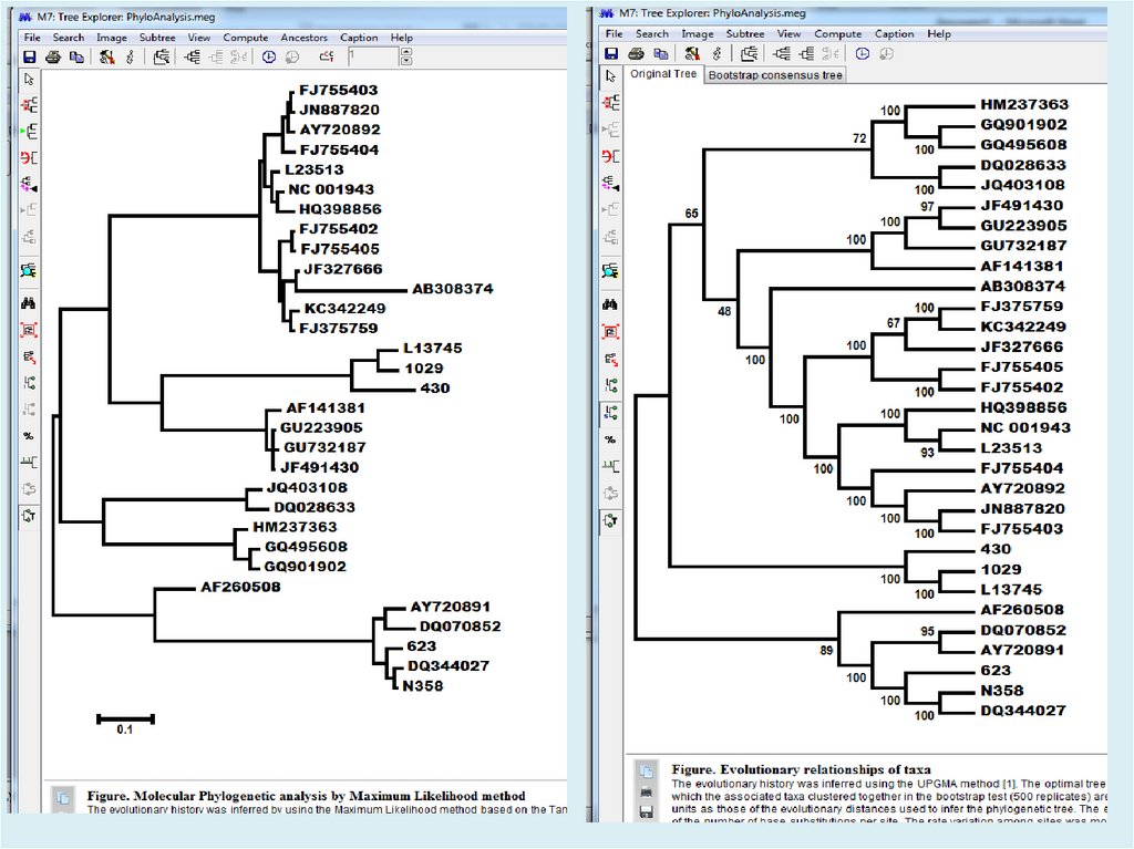
Figure. Evolutionary relationships of taxa
The evolutionary history was inferred using the
Neighbor-Joining method [1]. The optimal tree
with the sum of branch length = 2.17322002 is
shown. The percentage of replicate trees in
which the associated taxa clustered together in
the bootstrap test (500 replicates) are shown
next to the branches [2]. The tree is drawn to
scale, with branch lengths in the same units as
those of the evolutionary distances used to infer
the phylogenetic tree. The evolutionary distances
were computed using the Tamura-Nei method [3]
and are in the units of the number of base
substitutions per site. The rate variation among
sites was modeled with a gamma distribution
(shape parameter = 4). The differences in the
composition bias among sequences were
considered in evolutionary comparisons [4]. The
analysis involved 31 nucleotide sequences.
Codon positions included were
1st+2nd+3rd+Noncoding. All positions
containing gaps and missing data were
eliminated. There were a total of 2241 positions
in the final dataset. Evolutionary analyses were
conducted in MEGA7 [5].

23.

24.

25.

26.

27.

28.

91
86
8
50
10
0
L1374
100
100
86
62
10
0
99
100
66
6
0
10 100
0
5
HM
1029
JQ40
DQ
02
23
73
3108
86
3
63
GU223905
1430
08
56
02
49
Q
19
G
90
GQ
381
141
AF
2187
GU73
32
7
2
100
0
10
JF
5
08
43
61
100
JF49
37
4
0
26
83
100
56 100
100
100
30
8
AF
0
10
405
99
0
10
84
02
554
FJ7
9
75
5
37
49
FJ
2
2
34
C
K
AB
2
89
3
856
NC 001943
FJ755
3
40
0
72
35
1
40
4
D
07
Q
100
100
5
75
Y
L2
HQ3
98
75
5
100
FJ
A
FJ
62
3
AY
72
08
N358
DQ344027
820
887
JN
0.05
3

29.

30.

31.

32.

33.

34.

35. Newick tree format (Скобочная формула)

5.2
5.5
7.5
7.7
6.1
3.2
C
E
A
6.3
B
8.0
D
(((C,D),E)),(A,B));
только топология
(((C:3.2,D:8.0):5.5,E:7.7):5.2,(A:6.1,B:6.3):7.5);
длины ветвей

36.

37.

http://www.iqtree.org/