Financial Statement Analysis

1. Financial Statement Analysis

1
December 22

2. Financial Statement Analysis Contents

Overview and objective of financial statement analysis
Review and Re-formatting Statements for Financial Analysis
Income Statement – EBITDA and NOPLAT
Cash Flow Statement - Free Cash Flow and Equity Cash Flow
Financial ratio analysis
Management Performance
Valuation
Credit Analysis
Financial Model Drivers
Reference Slides
Financial Ratio Calculations
Discussion of Economic Profit
www.edbodmer.com
[email protected]
2 December 22

3. Financial Statement Analysis - Introduction

• Financial Statement Analysis should tell a story about the company –
How profitable is the company, what are the trends, how much risk is
there etc.
• You should be comfortable in reading various different financial
statements to be effective at financial modeling and financial analysis.
• Financial statement analysis is also important in:
Assessing management performance of a company and whether
projections of improvement or sustainability are reasonable.
Assessing the value of a company from historic performance.
Assessing the reasonableness of financial projections provided by a
company or the validity of earnings projections
Assessing whether the financial structure of a company is of
investment grade quality
www.edbodmer.com
[email protected]
3 December 22

4. Objectives of Financial Statement Analysis

• Financial statement analysis is like detective work – How can we use
information in financial statements to make assessments of various
issues. The financials should paint a picture of what has happened to
the company:
How can we quickly review the income statement, balance sheet
and cash flow statement to determine how the stock market value of
a company compares to inherent value.
How can we look the financial statements and assess risks
associated with a company and whether the company has sufficient
cash flow to pay off debt.
Finance and valuation are about projecting the future -- how can
financial statement analysis be used in making projections.
The problem in any financial analysis and valuation is that
measuring risk is very difficult
www.edbodmer.com
[email protected]
4 December 22

5. Double Counting and Judgments in Financial Ratio Analysis

In analyzing financial statements judgments must be made in computing key data
such as EBITDA and in developing financial ratios.
Examples
Whether or not to include Other Income in EBITDA
o If other income not in EBITDA, then should not add non-consolidated
subsidiary companies in invested capital
Exploration Expenses taken out of EBITDA
o Make consistent between companies with different accounting policies
Goodwill (ROIC with or without goodwill depending on analysis issue)
Minority Interest (if include or exclude do for both income and balance)
o Total of minority interest is in EBITDA, therefore must include
financing of minority interest in invested capital
A key principle is that the financial data and the financial ratios are consistent and
logical – work through simple examples
www.edbodmer.com
[email protected]
5 December 22

6. Income Statement

6
December 22

7. Income Statement

Review trends in EBITDA, EBIT, EBT and Net Income and explain what is
happening to the company
EBITDA includes operating earnings and other income, but it does not include
foreign exchange gains or losses, minority interest, extraordinary income or
interest income.
EBITDA is a rough proxy for free cash flow
EBITDA is not generally shown on Income Statement
Potential Adjustments for items such as exploration expense
Compare EBIT to Net Assets and Net Capital
Ratio of EBITDA to Revenues should be shown for historic and projected periods
EBITDA is related to un-levered cash flow while Net Income and EPS are after
leverage
NOPLAT is computed by EBIT less adjusted taxes, where taxes are computed
through adjusting income taxes.
www.edbodmer.com
[email protected]
7 December 22

8. Standard Computation of EBITDA

www.edbodmer.com
[email protected]
8 December 22

9. Problems with EBITDA

• EBITDA is useful in its simplicity, and can be a good reference for
comparison of debt and value, but it has weaknesses:
EBIT is more important than DA, because must use cash for
replacing depreciation and amoritsation
In credit analysis, EBITDA works better for low rated credits than
high rated credits. (Moody’s)
EBITDA is a better measure for companies with long-lived assets
EBITDA can be manipulated through accounting policies (operating
expenses versus capital expenditures)
EBITDA ignores changes in working capital, does not consider
required re-investment, says nothing about the quality of earnings,
and it ignores unique attributes of industries.
www.edbodmer.com
[email protected]
9 December 22

10. Simplified Income Statement

Sales
COGS
=
-
Gross Margin
SG&A
Other Expenses
+
Other Income
=
EBITDA
-
Depreciation and Amortization
=
EBIT
-
Interest Expense (income)
=
-
EBT
Income Taxes
-
Minority Interest
=
Net Income
There is a debate about how to handle
other income from non-consolidated
subsidiary companies.
One school of thought (McKinsey) is that
they should be valued separately since
they will have different cost of capital etc.
In this case, do not include in EBITDA
and remove the asset balance from the
invested capital. Must be consistent
NOPLAT = EBIT x (1-tax rate)
NOPLAT = Net Income + Interest Expense x (1-tax)
www.edbodmer.com
[email protected]
10December 22

11. Analysis of Income Statement – Computation of EBITDA, Minority Interest, Preferred Dividends, Exploration Expense

www.edbodmer.com
[email protected]
11 December 22

12. Income Statement Analysis

Example of Adjustments to EBITDA
Exploration Expenses (EBITDAX)
Rental and Lease Payments (EBITDR)
EBITDA Computation
Top Down – move other income
Bottom-up (Indirect)
EBITDA Notes
Interest Income out of EBITDA
Interest Expense not in EBITDA
Understand Non-cash Expenses
o Deferred Mining Costs
o Equity Income
o Minority Interest
www.edbodmer.com
[email protected]
12December 22

13. Discounted Cash Flow Analysis – Real World Example

Credit Suisse First Boston estimated the present value of the stand-alone,
Unlevered, after-tax free cash flows that Texaco could produce over calendar
years 2001 through 2004 and that Chevron could produce over the same period.
The analysis was based on estimates of the managements of Texaco and
Chevron adjusted, as reviewed by or discussed with Texaco management, to
reflect, among other things, differing assumptions about future oil and gas prices.
Ranges of estimated terminal values were calculated by multiplying estimated
calendar year 2004 earnings before interest, taxes, depreciation, amortization and
exploration expense, commonly referred to as EBITDAX, by terminal EBITDAX
multiples of 6.5x to 7.5x in the case of both Texaco and Chevron.
The estimated un-levered after-tax free cash flows and estimated terminal values
were then discounted to present value using discount rates of 9.0 percent to
10.0 percent.
That analysis indicated an implied exchange ratio reference range of 0.56x to
0.80x.
www.edbodmer.com
[email protected]
13December 22

14. Employee Stock Options

• One can debate the treatment of employee stock options for EBITDA,
free cash flow and valuation.
• Think of options as giving stock to employees
If the treatment has changed over the years and it is a significant
expense, make adjustments to current or prior statements for
consistency.
Think of options as giving free shares to employees. The value of
existing shareholders is diluted.
o One can argue that this is two things
First, employees are compensated and the cash should be
accounted for
Second, invested capital is increased and the new equity
should be included in the capital base
www.edbodmer.com
[email protected]
14December 22

15. Cash Flow Statement

15 December 22

16. Cash Flow Statement

Modern Cash Flow Statement has separation between
Operations
Capital expenditures (to maintain and grow operations) and
Financing
Operating Cash Flow
Add back items from the income statement that do not use cash
(depreciation, dry hole costs etc)
Analyze how much cash flow the company generated and how it raised funds or
disposed funds
Use Cash Flow statement as a basis to compute free cash flow although cash flow
not presented on the statement
Problem: Interest Expense – related to financing and not operations – is in
the Net Income and is included in Cash From Operations
www.edbodmer.com
[email protected]
16December 22

17. Cash Flow Statement

A. Operating Cash Flows
1) Net Income including interest expense, interest income and taxes
2) Depreciation
3) Deferred Taxes
4) Working Capital Changes
5) Minority Interest on Income Statement and Other Items
B. Investing Cash Flows
1) Capital Expenditure and Asset Purchases
3) Sale of Property, Plant, & Equipment
4) Inter-Corporate Investment
C. Financing Cash Flows
1) Dividend Payments
3) Proceeds from Equity or Debt Issuance
4) Equity Repurchased
5) Debt Principal Payments
www.edbodmer.com
[email protected]
17December 22

18. Cash Flow Statement Example

www.edbodmer.com
[email protected]
18December 22

19. The Notion of Free Cash Flow

• In practice the term cash flow has many uses. For example, operating
cash flow is net income plus depreciation.
• Free cash flow is the cash flow that is available to investors – FREE of
obligations such as capital expenditures and taxes -- to both debt and
equity investors – after re-investing in plant, and financing and paying
taxes.
• Accountants define cash flow from operations as net income plus
depreciation and other non-cash items less changes in working capital.
However, this cash flow is not available for distribution to equity holders
and debt holders. The free cash flow must account for capital
expenditures, repayments of debt, deferred items and other factors.
• Free cash flow consists of
Cash flow to equity holders
Cash flow to debt holders
www.edbodmer.com
[email protected]
19December 22

20. Theoretical Context – Miller and Modigliani

• Theory that changed finance in 1958
Value assets on fundamental operating characteristics such as the
capacity utilisation, the cost and the efficiency of assets and not the
manner in which assets are financed – debt versus equity or the
manner in which assets are hedged.
This has led to the discounted cash flow model that underlies most
valuations
The proof was based on a simple arbitrage idea that you could buy
stock in a company that has no debt and then borrow against the
stock. This will yield the same results as if the company borrowed
money instead of you.
The implication of this is that project finance is irrelevant
www.edbodmer.com
[email protected]
20December 22

21. Fundamental Distinction in Financial Analysis – Free Cash Flow and Equity Cash Flow

• Free Cash flow that is independent from financing
Valuation
Performance in managing assets
Claims on free cash flow
Cash flow to pay debt obligations
Comparisons unbiased by capital structure policy
• Equity cash flow
Valuation of equity securities
Performance for shareholders
www.edbodmer.com
[email protected]
21December 22

22. Importance of Free Cash Flow

Alternative Definitions, but one correct concept
Free Cash Flow Is Also Known As Unleveraged Cash Flow
Unleveraged Cash Flow Is Not Distorted By The Capital Structure
Free Cash Flow should not change when the capital structure changes
Free Cash Flow should be the same as equity cash flow if no debt is
outstanding and not cash balances are built up.
Free Cash Flow in Valuation
PV of Free Cash Flow Defines Enterprise Value
The Relevant Discount Rate Is The Unlevered Discount Rate or the
Weighted Average Cost of Capital
IRR on Free Cash Flow is the Project IRR
Free Cash Flow in Economic Value
FCF – Carrying Charge = Economic Profit
www.edbodmer.com
[email protected]
22December 22

23. Cash Flow Statement in Financial Model

Analysis in Cash Flow Statements
Compute Cash Flow before Financing
o Operating Cash Flow minus Capital Expenditures
o Use Cash Flow Before Financing in Deriving Free Cash Flow
Equity Cash Flow
o Dividends less Cash Investments
o Cash Flow Before Financing less Maturities plus New Debt Issues
Last Line on Cash Flow Statement Includes
o Change in Cash Balance
o Change in Short-term Debt or Overdrafts
o Beginning Balance + Change = Ending Cash
o Beginning Balance of STD + Change = Ending Short-term Debt
www.edbodmer.com
[email protected]
23December 22

24. Free Cash Flow Formulas

Free cash flow can be computed from the income statement or from the cash flow statement.
From the cash flow statement, the formula is:
Cash Before Financing
Plus: Interest Expense
Less: Tax Shield on Interest
From the income statement, the formula is:
EBITDA
Some argue that free cash flow
should not include non-operating
items. Here the non-consolidated
companies are treated in a similar
manner as liquid investments
Less: Taxes on EBIT
Less: Working Capital Investment
Less: Capital Expenditures
From Net Income
Net Income
Add: Net of Tax Interest
Add Depreciation, Deferred Taxes and Other Non-Cash Changes
Less: Changes in Working Capital
Less: Capital Expenditures
www.edbodmer.com
[email protected]
24December 22

25. Free Cash Flow from NOPLAT

Free cash flow can be computed using the notion of net operating profit less
adjusted tax as follows (assuming no extraordinary income)
Step 1: Compute NOPLAT
Net Income
Plus Net Interest after Tax
Plus Deferred tax
Equals NOPLAT
Step 2: Compute Free Cash Flow
NOPLAT
Plus: Depreciation
Less: Change in Working Capital
Less: Capital Expenditures
Equals Free Cash Flow
www.edbodmer.com
[email protected]
25December 22

26. Free Cash Flow Example

One could make adjustments for
dividends payable, interest payable and
other items in the working capital
analysis.
In actual situations,
must adjust the free
cash flow for deferred
tax
www.edbodmer.com
[email protected]
26December 22

27. Balance Sheet

27 December 22

28. Balance Sheet Adjustments

When analysing the balance sheet, various items should be adjusted and grouped
together:
Net Debt
o Total short and long term debt minus liquid investments held and
surplus cash
Cash Bucket
o For modelling, subtract short-term debt from surplus cash and liquid
investments
Surplus Cash
o Include temporary investments and also include long-term investments
Current Assets and Current Liabilities
o Separate the surplus cash from current assets and the debt from
current liabilities and relate remaining working capital items to revenue
and expense items
www.edbodmer.com
[email protected]
28December 22

29. Balance Sheet Issues

• Treat surplus cash as negative debt and debt as negative cash
Rule of thumb – cash is 2% of revenues
Example – when developing a basic cash flow model, group the
cash and the debt as one account and then separate this account
on the balance sheet.
Unfunded pension expenses should be treated like debt – they
involve a fixed obligation and they can be replaced with debt when
they are funded.
Deferred taxes depend on the way deferred taxes are modelled for
cash flow purposes. If you model future changes in deferred taxes
and take account of these in projections, do not put deferred taxes
as a component of equity.
www.edbodmer.com
[email protected]
29December 22

30. Problems with Equity Balance

• Would like the return on equity and the return on invested capital to
measure equity invested by shareholders for return on investment and
return on equity
Problems with using equity balance on the balance sheet to
measure equity investment
o Write-offs of plant
o Accumulated Other Comprehensive Income
o Goodwill
o Re-structuring losses
o Employee Stock options
Can make adjustments to equity balance
www.edbodmer.com
[email protected]
30December 22

31. Financial Ratio Analysis

31 December 22

32. Tension between Equity Analysis and Asset Analysis

Free Cash Flow
Equity Cash Flow
Project IRR
Equity IRR
ROIC (ROCE)
ROE
WACC
Cost of Equity
Enterprise Value
Market Capitalisation
EV/EBITDA
P/E
Market to Replacement Cost
Market to Book Ratio
EV = Σ Value of Business Units = Debt + Equity Value
In ratio analysis, cash = negative debt
www.edbodmer.com
[email protected]
32December 22

33. IRR Mathematics and IRR Exercise

Why we raise to a
power with two year
Example: Invest 100 and receive 120 in 1 year case
• IRR is simply rate of return
IRR = 120/100 = 120% - 100% = 20%
• If the cash flow is over two years
FV = PV (1+r) (1+r)
FV = PV (1+r)2
IRR = -100 , 60 , 60 13.07%
FV/PV = (1+r)2
Modified IRR with 5% Re-investment
(FV/PV)^(1/2) = (1+r)
60 receives 5% in year two 60 x (1.05) = 63 (FV/PV)^(1/2) – 1 = r
Plus final 60 = 123
MIRR = (123/100)^(1/2) - 1 = 10.9%
www.edbodmer.com
[email protected]
33December 22

34. Financial Ratio Analysis

Purpose :
Evaluate relation between two or more economically important items (one is
the starting point for further analysis)
Cautions:
Accounting analysis is important (deferred taxes etc.)
Interpretation is key
What does the P/E mean
Is an interest coverage of 3.5 good
Why is the ROIC low
Should we use MB, PE or EV/EBITDA
Document financial ratios (numerator and denominator) with footnotes and
comments
Show components of numerator and denominator in rows above the ratio
calculation
www.edbodmer.com
[email protected]
34December 22

35. General Discussion of Financial Ratios

Financial Ratios Often Compares Income Statement or Cash Flow with Balance
Sheet
In developing ratios, understand why the formula is developed (e.g. other
income and other investments in return on invested capital)
There is Not Necessarily One Single Correct Formula
For example, pre-tax or after-tax return on assets.
Keep the numerator consistent with the denominator
Financial Ratios should be evaluated in the context of benchmarks
Credit ratios and bond rating standards
Returns and cost of capital
Operating ratios and history
www.edbodmer.com
[email protected]
35December 22

36. Classes of Financial Ratios

Management Performance
Ratios that measure the historic economic performance of management and
evaluate whether the economic performance can be maintained (e.g. ROIC)
Valuation
Ratios that are used to give an indication of the value of the company (e.g.
P/E)
Credit Analysis
Ratios that gauge the credit quality and liquidity of the company (e.g.
Interest coverage and current ratio)
Model Evaluation
Ratios used to evaluate the assumptions and mechanics of financial
forecasts
www.edbodmer.com
[email protected]
36December 22

37. Ratios that Measure Management Performance

37 December 22

38. Class 1: Financial Indicators of Management Performance

Evaluate Whether Management is Doing a Good Job with Investor Funds (Not if
the company is appropriately valued)
Return on Invested Capital
Return on Assets
Return on Equity
Market/Book Ratio
Market Value/Replacement Cost
Key Issue
Evaluate relative to risk
o ROE versus Cost of Equity
o ROIC versus WACC
www.edbodmer.com
[email protected]
38December 22

39. ROIC, WACC and Growth

• ROIC is before interest and the return covers both debt and equity
financing – EBIT is before interest and investment includes both debt and
equity investment
• WACC is the blended average of debt and equity required returns
• ROIC versus WACC measures the ability to make true economic profit
• Once have economic profit, should grow the business as much as
possible.
www.edbodmer.com
[email protected]
39December 22

40. Basic Economic Principles, ROIC and Financial Analysis

• When you measure value, you are gauging the ability of a firm to realize
economic profit. For example, when you compare the equity IRR with the
equity cost of capital.
• When you assess assumptions in a financial forecast, you must assess
whether economic profit implicit in the assumptions can in fact be
realized. For example, if the financial forecast has a very high ROE, is
that reasonable.
• When you interpret financial statistics, you are gauging the strategy of the
company in terms of whether economic profit is being realized. In
reviewing the return on invested capital, does this demonstrate that the
company has the potential to earn economic profit.
www.edbodmer.com
[email protected]
40December 22

41. Return on Invested Capital Analysis

• ROIC is not distorted by the leverage of the company
• ROIC can be used to gauge economic profit and whether the company
should grow operations
• ROIC can be used to assess the reasonableness of projections
For example, if ROIC is very high and the company is in a
competitive business with few barriers to entry, the forecast is
probably not realistic.
• ROIC can be computed on a division basis EBIT and allocation of capital
to divisions from net assets to gauge the profit of parts of the company
• ROIC comes from sustainable competitive advantage and high market
share
www.edbodmer.com
[email protected]
41December 22

42. Formula for Return on Invested Capital

The return in invested capital formula can be for a division or an entire corporation. It is after
tax and after depreciation. Cash balances should be excluded from the denominator and
interest income from the numerator. Goodwill and goodwill amortization should be excluded.
Formula:
ROIC = EBITAT/Invested Capital
Where:
o EBITAT: Earnings before Interest Taxes and Goodwill Amortization less taxes on
EBITAT
o Taxes on EBITAT: Cash Income Taxes Less Tax on Interest Expense and
Interest Income and Tax on Non-operating Income
o Invested Capital less cash balance
Adjustments
Other Assets
Cash Balances
Goodwill
Other
www.edbodmer.com
[email protected]
42December 22

43. Issues in Management Performance Evaluation

Basic Formula: ROIC versus WACC
How to compute ROIC
o NOPLAT/Average Invested Capital
o May or may not include goodwill – If goodwill is not included, compute
NOPLAT without subtracting goodwill write-off and subtract net
goodwill from invested capital
o Reduce the invested capital by surplus cash balances
o Some don’t include other income – then the invested capital should be
reduced by other investments
o Can compute with ratios
EBIT Margin x (1-t) * Asset Turn
Asset Turn = Sales/Assets; EBIT Margin = EBIT/Sales
ROCE vs ROIC
o ROCE is generally computed in an indirect way by starting with net
income, and adding net of tax interest and adding minorities
www.edbodmer.com
[email protected]
43December 22

44. Exxon Mobil Return on Average Capital Employed

Return on average capital employed (ROCE) is a performance measure ratio.
From the perspective of the business segments, ROCE is annual business
segment earnings divided by average business segment capital employed
(average of beginning and end-of-year amounts).
These segment earnings include ExxonMobil’s share of segment earnings of
equity companies, consistent with our capital employed definition, and exclude
the cost of financing.
The corporation’s total ROCE is net income excluding the after-tax cost of
financing, divided by total corporate average capital employed. The corporation
has consistently applied its ROCE definition for many years and views it as the
best measure of historical capital productivity in our capital intensive longterm industry, both to evaluate management’s performance and to
demonstrate to shareholders that capital has been used wisely over the long
term. Additional measures, which tend to be more cash flow based, are used for
future investment decisions.
www.edbodmer.com
[email protected]
44December 22

45. Exxon Mobil Return on Capital Employed – Where are they making expenditures

www.edbodmer.com
[email protected]
45December 22

46. Exxon Mobil Return on Capital

2005
-millions of dollars
$ 36,130.00
Return on average capital employed
Net income
Financing costs -after tax
Third-party debt
ExxonMobil share of equity companies
All other financing costs – net -1
Total financing costs
2004
2003
25,330.00
$ 21,510.00
(1.00)
(144.00)
(295.00)
(137.00)
(185.00)
54.00
(69.00)
(172.00)
1,775.00
(440.00)
(268.00)
1,534.00
25,598.00
$ 19,976.00
36,570.00
$
Earnings excluding financing costs
$
Average capital employed
$ 116,961.00
$ 107,339.00
$ 95,373.00
31.30
23.80
20.90
Return on average capital employed – corporate total
(1)
www.edbodmer.com
$
“All other financing costs – net” in 2003 includes
interest income (after tax) associated with the
settlement of a U.S. tax dispute.
[email protected]
46December 22

47. Example of ROIC Calculation - AES

www.edbodmer.com
[email protected]
47December 22

48. Illustration of Invested Capital Computation

www.edbodmer.com
[email protected]
48December 22

49. ROE and ROIC – Note how to compute growth rates from ROE and Retention

www.edbodmer.com
[email protected]
49December 22

50. Example of Return on Capital Employed (Return on Invested Capital) in Financial Analysis

• The argument has been made that the best measure to evaluate management
performance that is not distorted by leverage (as in the case of ROE) or has the
problems of ROA is the return on invested capital. An example of use of this ratio is
in the Exxon Mobile Merger:
J.P. Morgan reviewed and analyzed the return on capital employed
("ROCE") of both Exxon and Mobil since 1993. J.P. Morgan observed that
Exxon's ROCE has consistently been 2-3% above that of Mobil.
J.P. Morgan's analysis indicated that if Mobil were to be merged with
Exxon, the combined entity's capital productivity would eventually be
higher than the pro forma capital productivity of Exxon and Mobil.
J.P. Morgan indicated that it would be reasonable to assume that the
benefits of this capital productivity increase would occur within three years of
the closing of the merger.
www.edbodmer.com
[email protected]
50December 22

51. Relationship Between Various Ratios and DuPont Analysis

Asset Utilization
Profitability
Gross Margin = Gross profit/ Sales
Less: Operating costs/ Sales
Equals EBIT Margin (EBIT/ Sales)
Working Capital/ Sales
Plus:
Long-term capital/ Sales
Equals:Capital employed/ Sales
1 divided by Capital Employed/ Sales
Equals: Asset Turnover
(Sales/ Capital Employed)
Multiplied by
ROCE(EBIT/ Capital Employed )
Multiplied by (1 minus Tax Rate)
ROCE(EBIT after Tax/ Capital Employed )
www.edbodmer.com
[email protected]
51December 22

52. Class 2: Financial Indicators of Market Value

Financial Ratios can be used to analyze whether the valuation of a company is
appropriate. Analysts should understand the drivers of different ratios. Valuation
Ratios include:
Universal Financial Ratios
o Price to Earnings Ratio
o Enterprise Value/EBITDA
o PEG (P/E to Earnings Growth) Ratio
o Market to Book Ratio
Industry Specific Financial Ratios
o Value/Reserve
o Value/Customer
o Value/Plane Seat
www.edbodmer.com
[email protected]
52December 22

53. Valuation Ratios and Benchmarks

• Valuation ratios measure the stock market value of a company relative to
some accounting measure such as EPS, EBITDA, Book Value/Share or
growth in EPS
• The ratios can be used as benchmarks in valuing non-traded companies
by using industry average valuation ratios.
• Example to value non-traded company:
Value of company = EPS of Company x Industry Average P/E Ratio
• Valuation ratios will be further discussed in the portion of the course
where corporate models are used to value companies.
www.edbodmer.com
[email protected]
53December 22

54. P/E Ratio

The P/E Ratio is the most prominent valuation ratio. It is affected by estimated
earnings growth, the ability of a company to earn economic profits and the growth
in profitable operations.
Formula:
Share Price/Earnings per Share
Issues
Trailing Twelve Months and Forward Twelve Months – Generally use
forward EPS
Formula: (1-g/r)/(k-g)
Problems
Affected by earnings adjustments
Causes too much focus on EPS
Distortions created by financing
www.edbodmer.com
[email protected]
54December 22

55. Illustration of EV Ratios and Computation of Market Value of Balance Sheet Components

www.edbodmer.com
[email protected]
55December 22

56. Investment Banker Analysis of Comparable Multiples

www.edbodmer.com
[email protected]
56December 22

57. Investment Banker Analysis of Multiples

www.edbodmer.com
[email protected]
57December 22

58. Use of PE in Valuation

• The long-run P/E ratio is often used in valuation. This process involves:
Project EPS
Compute Stable EPS
Compute P/E Ratio using formula
o P/E = (1-g/r)/(k-g)
o g – growth in EPS or Net Income
o r – rate of return earned on equity
o k – cost of equity capital
Related Formula for terminal value with NOPLAT (EBITAT)
o (1-g/ROIC)/(WACC – g)
The formula demonstrates where value really comes from
www.edbodmer.com
[email protected]
58December 22

59. Risk Assessment of Debt and Analysis of Credit Spreads

59 December 22

60. Liquidity and Solvency

Credit worthiness: Ability to honor credit obligations
(downside risk)
Liquidity
Solvency
Ability to meet short-term obligations
Focus:
• Current Financial
conditions
Ability to meet long-term
obligations
Focus:
• Current cash flows
• Long-term financial
conditions
• Liquidity of assets
• Long-term cash flows
• Extended profitability
www.edbodmer.com
[email protected]
60December 22

61. Solvency Ratios

Ratios are the center of traditional credit analysis that assesses whether a
company can re-pay loans. These ratios should be compared to benchmarks.
Solvency
o Debt Payback Ratios
Funds from Operations to Total Debt
Debt to EBITDA
o Leverage Ratios
Debt to Capital (Include Short-term Debt)
Market Debt to Market Capital
o Payment Ratios
Interest Coverage
Debt Service Coverage [Cash Flow/(Interest + Principal)]
o Capital Investment Coverage
Operating Cash Flow/Capital Expenditures
www.edbodmer.com
[email protected]
61December 22

62. Liquidity

Current Ratio
Current Assets to Current Liabilities
Current Assets less Inventory to Current Liabilities
Model Working Capital
Current Assets less Cash and Temporary Securities minus Current liabilities
less Short-term Debt
Liquidity Assessment
Debt Profile (Maturities)
Bank Lines (Availability, amount, maturity, covenants, triggers)
Off Balance Sheet Obligations (Guarantees, support, take-or-pay contracts,
contingent liabilities)
Alternative Sources of Liquidity (Asset sales, dividend flexibility, capital
spending flexibility)
www.edbodmer.com
[email protected]
62December 22

63. Banks or Rating Agencies Value Debt with Risk Classification Systems

Map of Internal Ratings to Public Rating Agencies
Internal
Credit
Ratings
1
2
3
4
5
6
7
8
9
10
www.edbodmer.com
Code
Meaning
A
Exceptional
B
Excellent
C
Strong
D
Good
E
Satisfactory
F
Adequate
G
Watch List
H
Weak
I
Substandard
L
Doubtful
N
In Elimination
S
In Consolidation
Z
Pending Classification
Corresponding
Moody's
Aaa
Aa1
Aa2/Aa3
A1/A2/A3
Baa1/Baa2/Baa3
Ba1
Ba2/Ba3
B1
B2/B3
Caa - O
[email protected]
63December 22

64. S&P Ratio Definitions

S&P Ratio Definitions
www.edbodmer.com
[email protected]
64December 22

65. S&P Benchmarks

S&P Benchmarks
www.edbodmer.com
[email protected]
65December 22

66. Example of Using Ratios to Gauge Credit Rating

• The credit ratios are shown next to the achieved ratios. Concentrate on
Funds from operations ratios.
Note that based on business
profile scores published by
S&P
www.edbodmer.com
[email protected]
66December 22

67. Credit Rating Standards and Business Risk

Business Risk/Financial Risk
—Financial risk profile—
Business risk profile
Minimal Modest Intermediate Aggressive Highly leveraged
Excellent
AAA
AA
A
BBB
BB
Strong
AA
A
A-
BBB-
BB-
Satisfactory
A
BBB+
BBB
BB+
B+
Weak
BBB
BBB-
BB+
BB-
B
Vulnerable
BB
B+
B+
B
B-
Financial risk indicative ratios*
Minimal Modest Intermediate Aggressive Highly leveraged
Cash flow (Funds from operations/Debt) (%) Over 60
45–60
30–45
15–30
Below 15
Debt leverage (Total debt/Capital) (%)
Below 25 25–35
35–45
45–55
Over 55
Debt/EBITDA (x)
<1.4
1.4–2.0 2.0–3.0
3.0–4.5
>4.5
Key Industry Characteristics And Drivers Of Credit Risk
Credit risk impact: High (H); Medium (M); Low (L)
Risk factor
Industry
Airlines (U.S.)
Autos*
Auto suppliers*
High technology*
Mining*
Chemicals (bulk)*
Hotels*
Shipping*
Competitive power*
Telecoms (Europe)
Cyclicality
H
H
H
H
H
H
H
H
H
H
M
www.edbodmer.com
Competition
H
H
H
H
H
H
H
H
H
H
H
Capital intensity Technology risk
H
L
H
M
H
M
M
H
H
M
H
L
H
L
H
L
H
L
M
L
H
H
Regulatory/Gov
ernment
M/H
M
M
L
M/H
M
M
L
L
H
H
Energy
sensitivity
H
H
M
L/M
H
L
H
M
M
H
L
[email protected]
67December 22

68. Debt Capacity and Interest Cover

• Despite theory of
probability of default and
loss given default, the
basic technique to
establish bond ratings
continues to be cover
ratios,\.
www.edbodmer.com
[email protected]
68December 22

69. Default Rates and Credit Spreads

www.edbodmer.com
[email protected]
69December 22

70. Credit Spreads

Increase of 5%
www.edbodmer.com
Credit Crisis
[email protected]
70December 22

71. Moody’s Forecast of Default Rates

Defaults versus Long-term Average
Moody's Speculative Grade Trailing 12-Month Default Rates
Actual Jan. 2000 to Aug. 2002 / Forecasted Sept. 2002 to Feb. 2003
12.0%
11.0%
10.5%
9.6%
10.0%
9.0%
8.5%
7.7%
8.0%
7.0%
7.7%
8.8%
10.7%
10.5%
10.3% 10.3%
10.5%
10.3%
9.8%
10.1% 10.0% 10.0% 10.0% 10.0% 9.8%
9.3%
9.0%
8.8%
7.9%
7.1%
6.7%
6.2%
% 6.0%
5.0%
4.0%
3.77%*
3.0%
2.0%
1.0%
www.edbodmer.com
Note: *Long run annual default rate is 3.77%
Months
[email protected]
71December 22
Feb-03
Jan-03
Dec-02
Nov-02
Oct-02
Sep-02
Aug-02
Jul-02
Jun-02
May-02
Apr-02
Mar-02
Feb-02
Jan-02
Dec-01
Nov-01
Oct-01
Sep-01
Aug-01
Jul-01
Jun-01
May-01
Apr-01
Mar-01
Feb-01
Jan-01
0.0%

72. Updated Transition Matrix

www.edbodmer.com
[email protected]
72December 22

73. Probability of Default

• This chart shows rating migrations and the probability of default for
alternative loans. Note the increase in default probability with longer
loans.
www.edbodmer.com
[email protected]
73December 22

74. Bond Ratings and Historic Credit Spreads

www.edbodmer.com
[email protected]
74December 22

75. Credit Spreads for Utility Debt

www.edbodmer.com
[email protected]
75December 22

76. DSCR Criteria in Different Industries in Project Finance

Electric Power:
1.3-1.4
Resources:
1.5-2.0
Telecoms:
1.5-2.0
Infrastructure:
1.2-1.6
Minimum ratio could dip to 1.5
At a minimum, investment-grade merchant projects probably will have to exceed a
2.0x annual DSCR through debt maturity, but also show steadily increasing ratios.
Even with 2.0x coverage levels, Standard & Poor's will need to be satisfied that
the scenarios behind such forecasts are defensible. Hence, Standard & Poor's
may rely on more conservative scenarios when determining its rating levels.
For more traditional contract revenue driven projects, minimum base case
coverage levels should exceed 1.3x to 1.5x levels for investment-grade.
www.edbodmer.com
[email protected]
76December 22

77. Credit Spread on Debt Facilities

• The spread on a loan is directly related to the probability of default and
the loss, given default.
S
The Credit Triangle
S = P (1-R)
P
R
The credit spread (s) can be characterized as the default probability (P)
times the loss in the event of a default (R).
www.edbodmer.com
[email protected]
77December 22

78. Expected Loss Can Be Broken Down Into Three Components

Borrower Risk
EXPECTED
LOSS
$$
=
Probability of
Default
Facility Risk Related
Loss Severity
x
Given Default
Loan Equivalent
x
Exposure
(PD)
(Severity)
(Exposure)
%
%
$$
What is the probability
of the counterparty
defaulting?
If default occurs, how
much of this do we
expect to lose?
If default occurs, how
much exposure do we
expect to have?
The focus of grading tools is on modeling PD
www.edbodmer.com
[email protected]
78December 22

79. Comparison of PD x LGD with Precise Formula Case 1: No LGD and One Year

• .
www.edbodmer.com
[email protected]
79December 22

80. Comparison of PD x LGD with Precise Formula Case 2: LGD and Multiple Years

• .
Assumptions
Years
Risk Free Rate 1
Prob Default 1
Loss Given Default 1
5
5%
20.8%
80%
BB
PD
5
7
20.80%
Opening
100
Closing
127.63
Value
127.63
Risky - No Default
100
Prob
Closing
0.95
153.01
Value
145.36
Risky - Default
100
Alternative Computations of Credit Spread
Credit Spread 1
3.88%
PD x LGD 1
16.64%
Proof
Risk Free
Total Value
0.05
30.60
1.53
146.89
FALSE
Credit Spread Formula
With LGD
cs = ((1+rf)/((1-pd)+pd*(1-lgd))-rf)^(1/years)-1
www.edbodmer.com
[email protected]
80December 22

81. Default Rates by Industry

www.edbodmer.com
[email protected]
81December 22

82. Recovery Rates

www.edbodmer.com
[email protected]
82December 22

83. Mathematical Credit Analysis

83 December 22

84. General Payoff Graphs from Holding Investments with Future Uncertain Returns

Stock Payoff versus Price if Purchased or Sold Stock at $40
50
40
30
Payoff
20
10
Ending Stock Price
0
-10 0
10
20
30
40
50
60
70
80
-20
-30
-40
-50
www.edbodmer.com
Purchase at $40
Sell Stock Short
[email protected]
84December 22

85. Payoff Graphs from Call Option – Payoffs when Conditions Improve

Call Option Payoff Patterns
40
30
Payoff
20
10
0
-10
-20
0
20
Bought call
40
60
80
Ending Value
Sold Call
-30
-40
www.edbodmer.com
[email protected]
85December 22

86. Payoff Graphs from Buying Put Option – Returns are realized to buyer when the value declines

www.edbodmer.com
[email protected]
86December 22

87. Payoff Graphs from Selling Put Option – Value Changes with Value Decreases

Put Option Payoff Pattern from
Selling Put -- Lender Perspective
10
5
Payoff
0
-5 0
20
40
60
-10
80
100
120
Ending Firm Value
-15
-20
-25
-30
-35
-40
www.edbodmer.com
[email protected]
87December 22

88. The Black-Scholes/Merton Approach

Consider a firm with equity and one debt issue.
The debt issue matures at date T and has principal F.
It is a zero coupon bond for simplicity.
Value of the firm is V(t).
Value of equity is E(t).
Current value of debt is D(t).
www.edbodmer.com
[email protected]
88December 22

89.

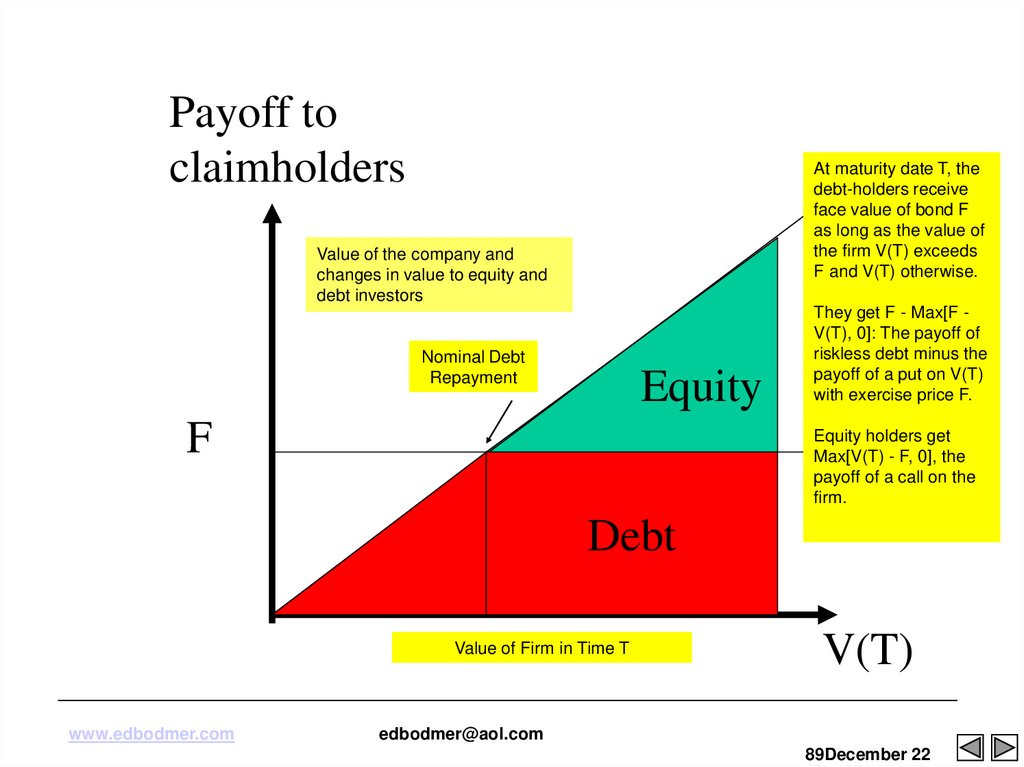
Payoff to
claimholders
At maturity date T, the
debt-holders receive
face value of bond F
as long as the value of
the firm V(T) exceeds
F and V(T) otherwise.
Value of the company and
changes in value to equity and
debt investors
Nominal Debt
Repayment
Equity
F
They get F - Max[F V(T), 0]: The payoff of
riskless debt minus the
payoff of a put on V(T)
with exercise price F.
Equity holders get
Max[V(T) - F, 0], the
payoff of a call on the
firm.
Debt
Value of Firm in Time T
www.edbodmer.com
V(T)
[email protected]
89December 22

90.

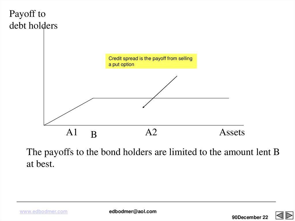
Payoff to
debt holders
Credit spread is the payoff from selling
a put option
A1
B
A2
Assets
The payoffs to the bond holders are limited to the amount lent B
at best.
www.edbodmer.com
[email protected]
90December 22

91. Merton’s Model

Merton’s model regards the equity as an option on the assets of the firm
In a simple situation the equity value is
max(VT -D, 0)
where VT is the value of the firm and D is the debt repayment required
Assumptions
Markets are frictionless, there is no difference between borrowing and
lending rates
Market value of the assets of a company follow Brownian Motion Process
with constant volatility
No cash flow payouts during the life of the debt contract – no debt repayments and no dividend payments
APR is not violated
www.edbodmer.com
[email protected]
91December 22

92. Merton‘s Structural Model (1974)

• Assumes a simple capital structure with all debt represented by one zero
coupon bond – problem in project finance because of amortization of
bonds.
• We will derive the loss rates endogenously, together with the default
probability
• Risky asset V, equity S, one zero bond B maturing at T and face value
(incl. Accrued interest) F
• Default risk on the loan to the firm is tantamount to the firm‘s assets VT
falling below the obligations to the debt holders F
• Credit risk exists as long as probability (V<F)>0
• This naturally implies that at t=0, B0<Fe-rT; yT>rf, where πT=yT-rf is the
default spread which compensates the bond holder for taking the default
risk
www.edbodmer.com
[email protected]
92December 22

93. Merton Model Propositions

Face value of zero coupon debt is strike price
Can use the Black-Scholes model with equity as a call or debt as a put option to directly
measure the value of risky debt
Can use to compute the required yield on a risky bond:
PV of Debt = Face x (1+y)^t
or
(1+y)^t = PV/Face
(1+y) = (PV/Face)^(1/t)
y = (PV/Face)^(1/t) – 1
With continual compounding = - Ln(PV/Face)/t
Computation of the yield allows computation of the required credit spread and computation of
debt value
Borrower always holds a valuable default or repayment option. If things go well repayment
takes place, borrower pays interest and principal keeps the remaining upside, If things go bad,
limited liability allows the borrower to default and walk away losing his/her equity.
www.edbodmer.com
[email protected]
93December 22

94. Default Occurs at Maturity of Debt if V(T)<F

Default Occurs at Maturity of Debt if V(T)<F
Asset Value
E (VT ) V0 e T
2
VT V0 exp{[ ]T T ZT }
2
VT
V0
F
Probability of default
T
www.edbodmer.com
Time
[email protected]
94December 22

95. Resources and Contacts

• My contacts
Ed Bodmer
Phone: +001-630-886-2754
E-mail: [email protected]
• Other Sources
Financial Library – project finance case studies including Eurotunnel
and Dabhol
Financial Library – Monte Carlo simulation analysis
www.edbodmer.com
[email protected]
95December 22