 Программирование
Похожие презентации:


")

")

")
")


Algorithms and data structures. Lecture 1. Introduction and Overview
1.
ALGORITHMSAND
DATA STRUCTURES
Introduction and Overview
◦ Yerasyl Amanbek
LECTURE #1
2.
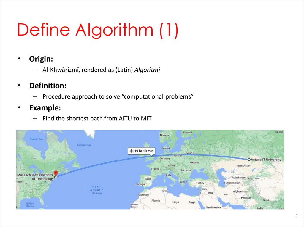
Define Algorithm (1)• Origin:
– Al-Khwārizmī, rendered as (Latin) Algoritmi
• Definition:
– Procedure approach to solve “computational problems”
• Example:
– Find the shortest path from AITU to MIT
2
3.
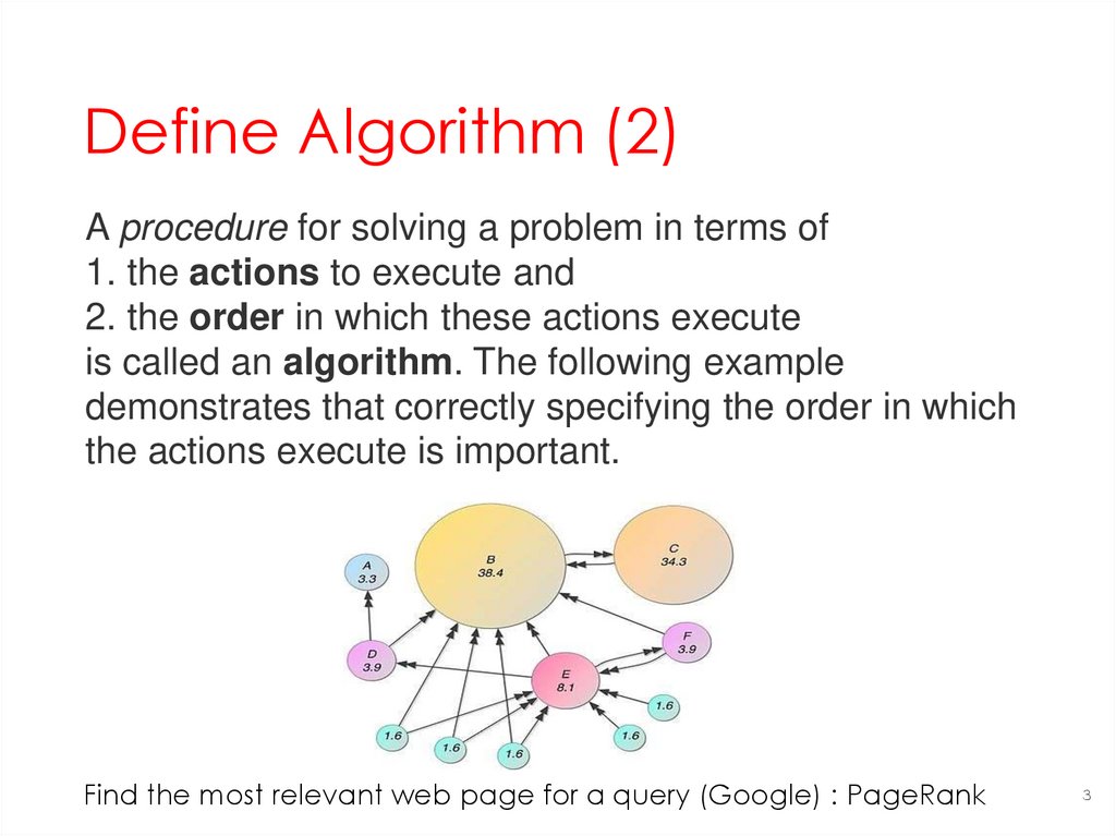
Define Algorithm (2)A procedure for solving a problem in terms of
1. the actions to execute and
2. the order in which these actions execute
is called an algorithm. The following example
demonstrates that correctly specifying the order in which
the actions execute is important.
Find the most relevant web page for a query (Google) : PageRank
3
4.
Main Features of an Algorithm• Various features
– Reusability/modularity
– Simplicity
– Memory footprint
– Speed
Algorithm is all about efficiency: Time vs. Space
Time complexity: Developing a formula for predicting how
fast and algorithm is, based on input size.
Space complexity: Developing a formula for predicting how
much memory an algorithm requires, based on input size.
Memory is extensible, time is not!
4
5.
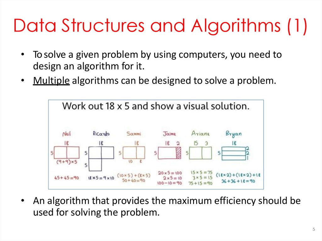
Data Structures and Algorithms (1)• To solve a given problem by using computers, you need to
design an algorithm for it.
• Multiple algorithms can be designed to solve a problem.
• An algorithm that provides the maximum efficiency should be
used for solving the problem.
5
6.
Data Structures and Algorithms (2)• The efficiency of and algorithm can be improved by using an
appropriate data structure.
• Data structures help in creating programs that are simple,
reusable, and easy to maintain.
• To solve a problem, you need a computer to write a program.
• A program is made up of two parts:
– Algorithm
– Data structures
• Arrays
• Queues
• Lists
• Linked Lists
• Trees
• Graphs
6
7.
Example of an AlgorithmConsider the “rise-and-shine algorithm” followed by one executive for getting
out of bed and going to work.
(1) Get out of bed;
(2) take off pajamas;
(3) take a shower;
(4) get dressed;
(5) eat breakfast;
(6) carpool to work.
This routine gets the executive to work well prepared to make critical
decisions. Suppose that the same steps are performed in a slightly
different order:
(1) Get out of bed;
(2) eat breakfast;
(3) take off pajamas;
(4) take a shower;
(5) Get dressed;
(6) carpool to work.
7
8.
Pseudocode• Informal language that helps to understand and develop
algorithms
• Pseudocode is similar to everyday language.
• Pseudocode:
Does not execute on computers
Help to “think out”
Can be easily converted to program
8
9.
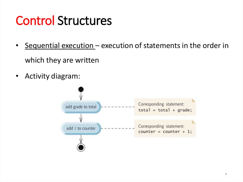
Control Structures• Sequential execution – execution of statements in the order in
which they are written
• Activity diagram:
9
10.
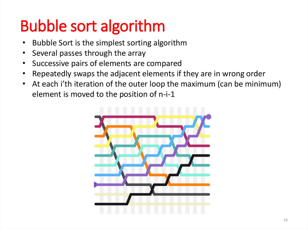
Bubble sort algorithmBubble Sort is the simplest sorting algorithm
Several passes through the array
Successive pairs of elements are compared
Repeatedly swaps the adjacent elements if they are in wrong order
At each i’th iteration of the outer loop the maximum (can be minimum)
element is moved to the position of n-i-1
10
11.
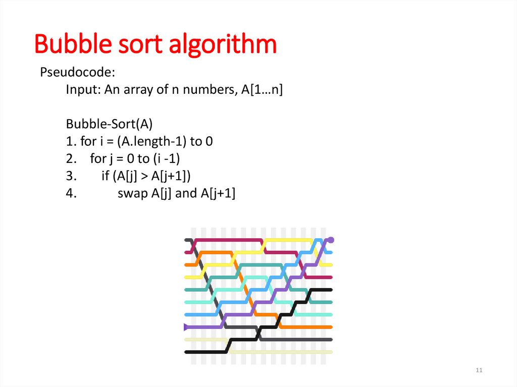
Bubble sort algorithmPseudocode:
Input: An array of n numbers, A[1…n]
Bubble-Sort(A)
1. for i = (A.length-1) to 0
2. for j = 0 to (i -1)
3.
if (A[j] > A[j+1])
4.
swap A[j] and A[j+1]
11
12.
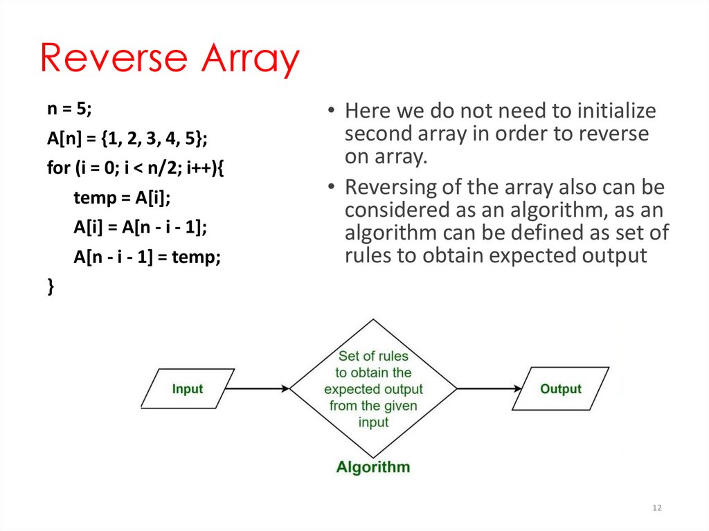
Reverse Arrayn = 5;
A[n] = {1, 2, 3, 4, 5};
for (i = 0; i < n/2; i++){
temp = A[i];
A[i] = A[n - i - 1];
A[n - i - 1] = temp;
}
• Here we do not need to initialize
second array in order to reverse
on array.
• Reversing of the array also can be
considered as an algorithm, as an
algorithm can be defined as set of
rules to obtain expected output
12
13.
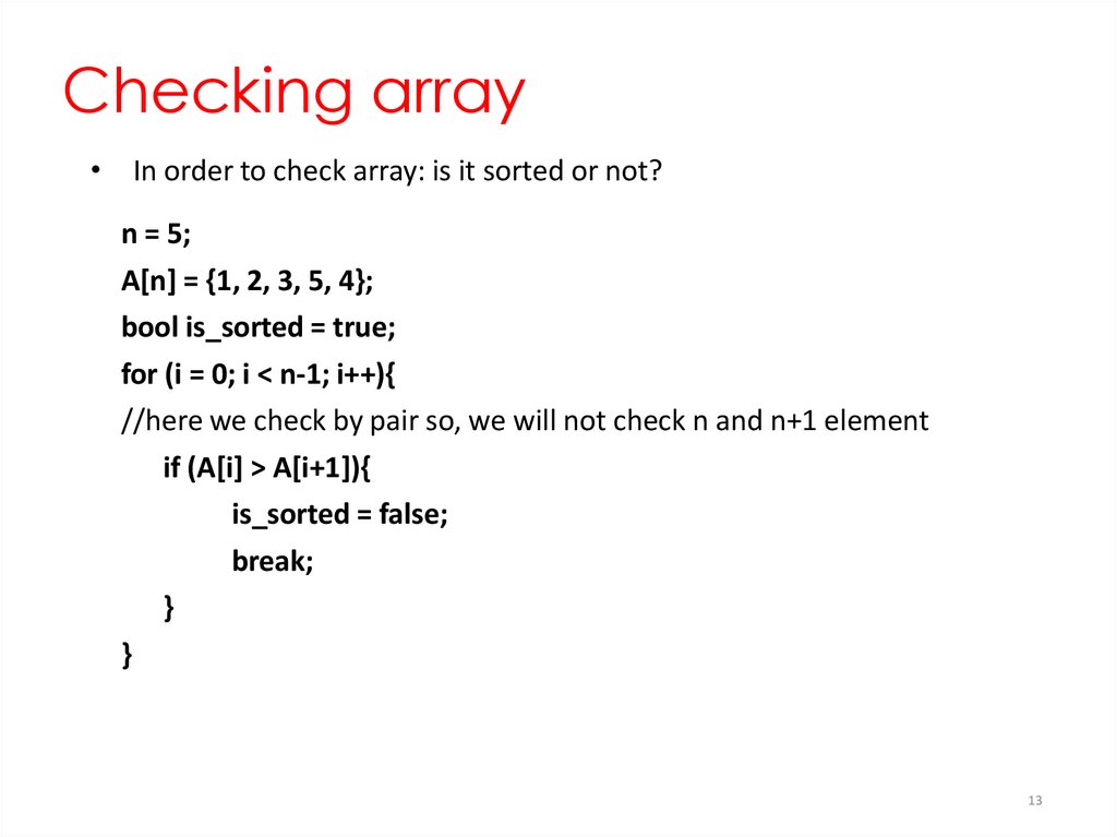
Checking array• In order to check array: is it sorted or not?
n = 5;
A[n] = {1, 2, 3, 5, 4};
bool is_sorted = true;
for (i = 0; i < n-1; i++){
//here we check by pair so, we will not check n and n+1 element
if (A[i] > A[i+1]){
is_sorted = false;
break;
}
}
13
14.
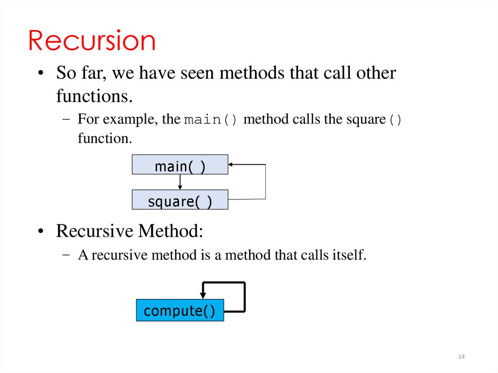
Recursion• So far, we have seen methods that call other
functions.
– For example, the main() method calls the square()
function.
main( )
square( )
• Recursive Method:
– A recursive method is a method that calls itself.
compute()
14
15.
Why we need Recursion?• Some problems are more easily solved by
using recursive functions.
• If you go on to take a computer science algorithms
course, you will see lots of examples of this.
• For example:
– Traversing through a directory or file system.
– Traversing through a tree of search results.
• For today, we will focus on the basic structure of
using recursive methods.
15
16.
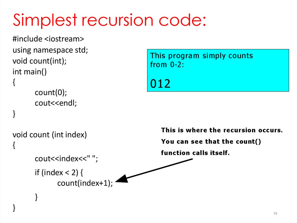
Simplest recursion code:#include <iostream>
using namespace std;
void count(int);
int main()
{
count(0);
cout<<endl;
}
void count (int index)
{
cout<<index<<" ";
This program simply counts
from 0-2:
012
This is where the recursion occurs.
You can see that the count()
function calls itself.
if (index < 2) {
count(index+1);
}
}
16
17.
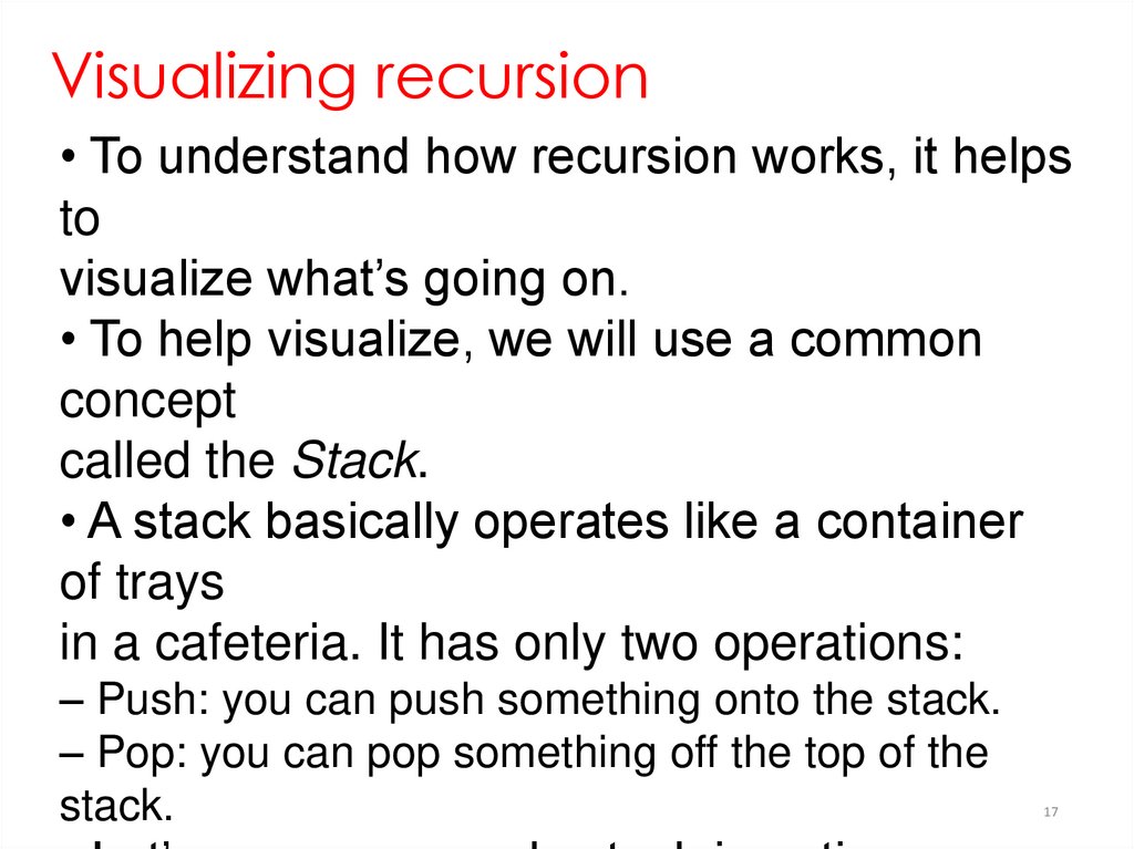
Visualizing recursion• To understand how recursion works, it helps
to
visualize what’s going on.
• To help visualize, we will use a common
concept
called the Stack.
• A stack basically operates like a container
of trays
in a cafeteria. It has only two operations:
– Push: you can push something onto the stack.
– Pop: you can pop something off the top of the
stack.
17
18.
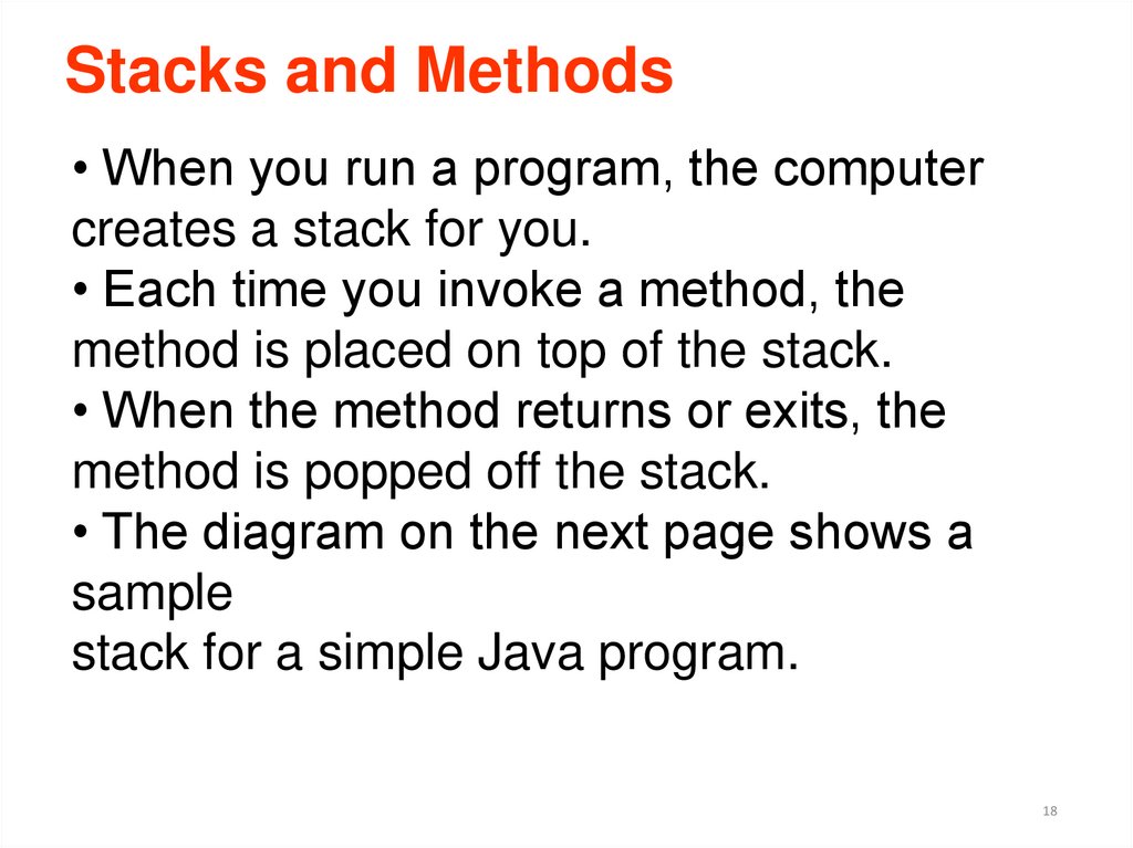
Stacks and Methods• When you run a program, the computer
creates a stack for you.
• Each time you invoke a method, the
method is placed on top of the stack.
• When the method returns or exits, the
method is popped off the stack.
• The diagram on the next page shows a
sample
stack for a simple Java program.
18
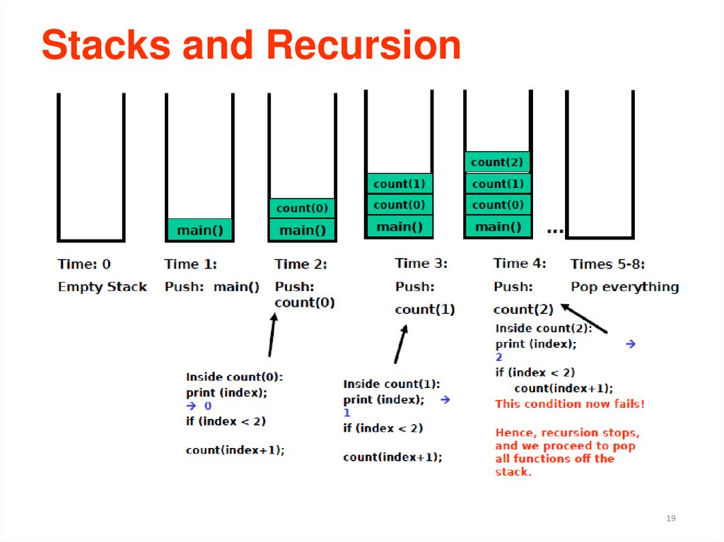
19.
Stacks and Recursion19
20.
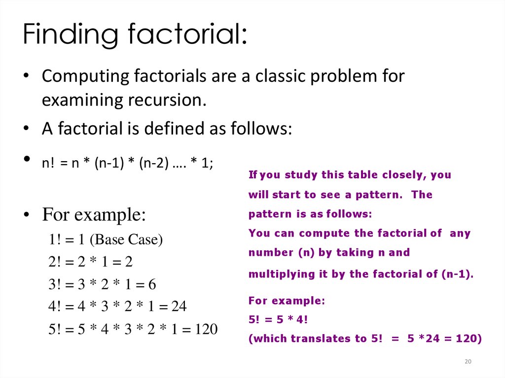
Finding factorial:• Computing factorials are a classic problem for
examining recursion.
• A factorial is defined as follows:
• n! = n * (n-1) * (n-2) …. * 1;
If you study this table closely, you
will start to see a pattern. The
• For example:
1! = 1 (Base Case)
2! = 2 * 1 = 2
3! = 3 * 2 * 1 = 6
4! = 4 * 3 * 2 * 1 = 24
5! = 5 * 4 * 3 * 2 * 1 = 120
pattern is as follows:
You can compute the factorial of any
number (n) by taking n and
multiplying it by the factorial of (n-1).
For example:
5! = 5 * 4!
(which translates to 5! = 5 * 24 = 120)
20
21.
Seeing the Pattern• Seeing the pattern in the factorial example is
difficult at first.
• But, once you see the pattern, you can apply
this pattern to create a recursive solution to the
problem.
• Divide a problem up into:
– What it can do (usually a base case)
– What it cannot do
• What it cannot do resembles original problem
• The function launches a new copy of itself
(recursion step) to solve what it cannot do.
21
22.
Recursion vs. Iteration• Iteration
– Uses repetition structures (for, while or
do…while)
– Repetition through explicitly use of repetition
structure
– Terminates when loop-continuation condition
fails
– Controls repetition by using a counter
• Recursion
– Uses selection structures (if, if…else or switch)
– Repetition through repeated method calls
– Terminates when base case is satisfied
– Controls repetition by dividing problem into
22
23.
Recursion vs. Iteration (cont.)• Recursion
– More overhead than iteration
– More memory intensive than iteration
– Can also be solved iteratively
– Often can be implemented with only a few lines
of code
23