Lecture_1_ASD_Bekarystankyzy (1)

1.

Data Structures and Algorithms
Lecture 1: Introduction. What is
Algorithm. Notation
Lecturer:Bekarystankyzy Akbayan, PhD
1

2.

In Computer Science, an algorithm is a finite set of instructions,
used to solve problems or perform tasks, based on the
understanding of available alternatives.
https://msoe.us/taylor/tutorial/ce2810/csimila
r

3.

Moving From Java to C++
https://people.eecs.ku.edu/~jrmiller/Courses/JavaToC++/Arrays.html
Principal differences between Java & С++:
https://blog.ithillel.ua/ru/articles/raznica-mezhdu-yazykamiprogrammirovaniya-c-i-java

4.

Language History C Family
The C language was developed at AT & T in the early 1970s.
C is still very popular in a number of domains including operating system development and embedded systems.
Compiler generates machine code that runs on specific microcontrollers.
The C++ language was developed at Bell Labs in 1979 (originally named "C with Classes").
Attempts to be backwards compatible with C.
Adds a number of features including object oriented constructs like user defined classes.
Compiler generates machine code that runs on specific microcontrollers.
Java was developed at Sun Microsystems and released in 1995.
Was designed so that C/C++ developers could quickly learn.
Uses very similar syntax as C/C++.
Compiler produces byte code that runs on a Java Virtual Machine.
Includes a number of language "improvements" over C++.
C# was developed at Microsoft beginning in 1999.
Similar to Java but compiler produces byte code (termed Common Intermediate Language) that runs on the .NET runtime.
Includes a number of language "improvements" over Java.

5.

Complexity
Reading: Carrano, section 9.1.
• Asymptotic Analysis
5

6.

Introduction to Asymptotic analysis
Algorithmic complexity is a very important topic in
computer science. Knowing the complexity of
algorithms allows you to answer questions such as:
• How long will a program run on an input?
• How much space will it take?
• Is the problem solvable?
6

7.

The running time of programs
1. We would like an algorithm that is easy to
understand, code, and debug.
2. We would like an algorithm that makes
efficient use of the computer's resources,
especially, one that runs as fast as possible.
7

8.

Measuring the Running Time of a
Program
The running time of a program depends on factors such
as:
1. the input to the program,
2. the quality of code generated by the compiler
used to create the object program,
3. the nature and speed of the instructions on the
machine used to execute the program,
4. the time complexity of the algorithm underlying
the program.
8

9.

Central topic
The comparison of algorithm is a central topic
to computer science.
The analysis of algorithm is the area of
computer science that provide tools for
contrasting efficiency of different algorithms.
9

10.

Asymptotic Analysis
• Names for classes of algorithms:
constant
logarithmic
polylogarithmic
linear
<“en log en”>
quadratic
cubic
polynomial
exponential
(n0) = (1)
(lgn)
(lgkn), k ≥ 1
(n)
(nlgn)
(n2)
(n3)
(nk), k ≥ 1
(an), a > 1
Growth
Rate
Increasing
10

11.

Basic asymptotic efficiency classes
Class
Name
Comments
1
Constant
Algorithm ignores input
(i.e., can’t even scan input)
lgn
Logarithmic
Cuts problem size by constant fraction on
each iteration
n
Linear
Algorithm scans its input (at least)
nlgn
“n-log-n”
Some divide and conquer
n2
Quadratic
Loop inside loop = “nested loop”
n3
Cubic
Loop inside nested loop
2n
Exponential
Algorithm generates all subsets of
n-element set
n!
Factorial
Algorithm generates all permutations of
n-element set
11

12.

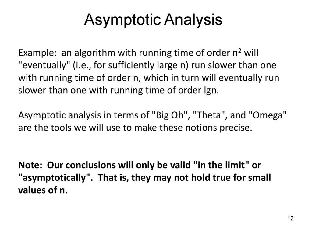
Asymptotic Analysis
Example: an algorithm with running time of order n2 will
"eventually" (i.e., for sufficiently large n) run slower than one
with running time of order n, which in turn will eventually run
slower than one with running time of order lgn.
Asymptotic analysis in terms of "Big Oh", "Theta", and "Omega"
are the tools we will use to make these notions precise.
Note: Our conclusions will only be valid "in the limit" or
"asymptotically". That is, they may not hold true for small
values of n.
12

13.

Asymptotic Analysis
• Classifying algorithms is generally done in terms of worstcase running time:
– O (f(n)): Big Oh--asymptotic upper bound.
(f(n)): Big Omega--asymptotic lower bound
(f(n)): Theta--asymptotic tight bound
13

14.

14

15.

15

16.

16

17.

"Big Oh" - Upper Bounding Running Time
Definition: f(n) O(g(n)) if there exist constants c > 0 and
n0 > 0 such that
f(n) cg(n) for all n ≥ n0.
Intuition:
• f(n) O(g(n)) means f(n) is “of order at most”, or “less than or
equal to” g(n) when we ignore small values of n and constants
• f(n) is eventually trapped below (or = to) some constant multiple
of g(n)
• some constant multiple of g(n) is an upper bound for f(n)
(for large enough n)
17

18.

Example
One important advantage of big-O notation is that it
makes algorithms much easier to analyze, since we can
conveniently ignore low-order terms.
An algorithm that runs in time:
10n3 + 24n2 + 3n log n + 144
is still a cubic algorithm, since
10n3 + 24n2 + 3n log n + 144
<= 10n3 + 24n3 + 3n3 + 144n3
<= (10 + 24 + 3 + 144)n3
= O(n3).
18

19.

19

20.

20

21.

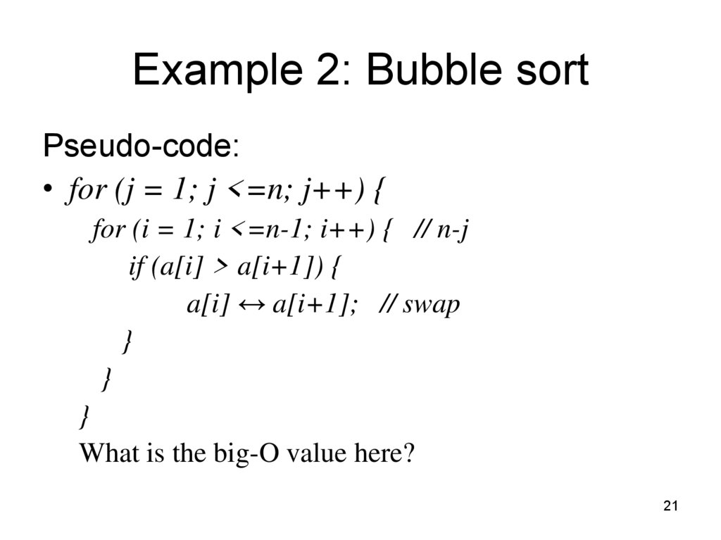
Example 2: Bubble sort
Pseudo-code:
• for (j = 1; j <=n; j++) {
for (i = 1; i <=n-1; i++) { // n-j
if (a[i] > a[i+1]) {
a[i] ↔ a[i+1]; // swap
}
}
}
What is the big-O value here?
21

22.

Confused?
Basic idea: ignore constant factor
differences and lower-order terms
• 617n3 + 277x2 + 720x + 7x = ?
•2=?
• sin(x) = ?
22

23.

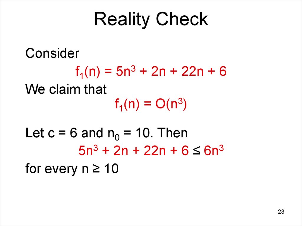
Reality Check
Consider
f1(n) = 5n3 + 2n + 22n + 6
We claim that
f1(n) = O(n3)
Let c = 6 and n0 = 10. Then
5n3 + 2n + 22n + 6 ≤ 6n3
for every n ≥ 10
23

24.

Reality Check (Part Two)
If
f1(n) = 5n3 + 2n + 22n + 6
we have seen that
f1(n) = O(n3)
but f1(n) is not O(n2), because no
positive value for c or n0 works!
24

25.

Logarithms
The big-O interacts with logarithms in a
particular way.
logb n = log2 n
log2 b
– changing b changes only constant factor
– When we say f(n) = O(log n), the base is
unimportant
25

26.

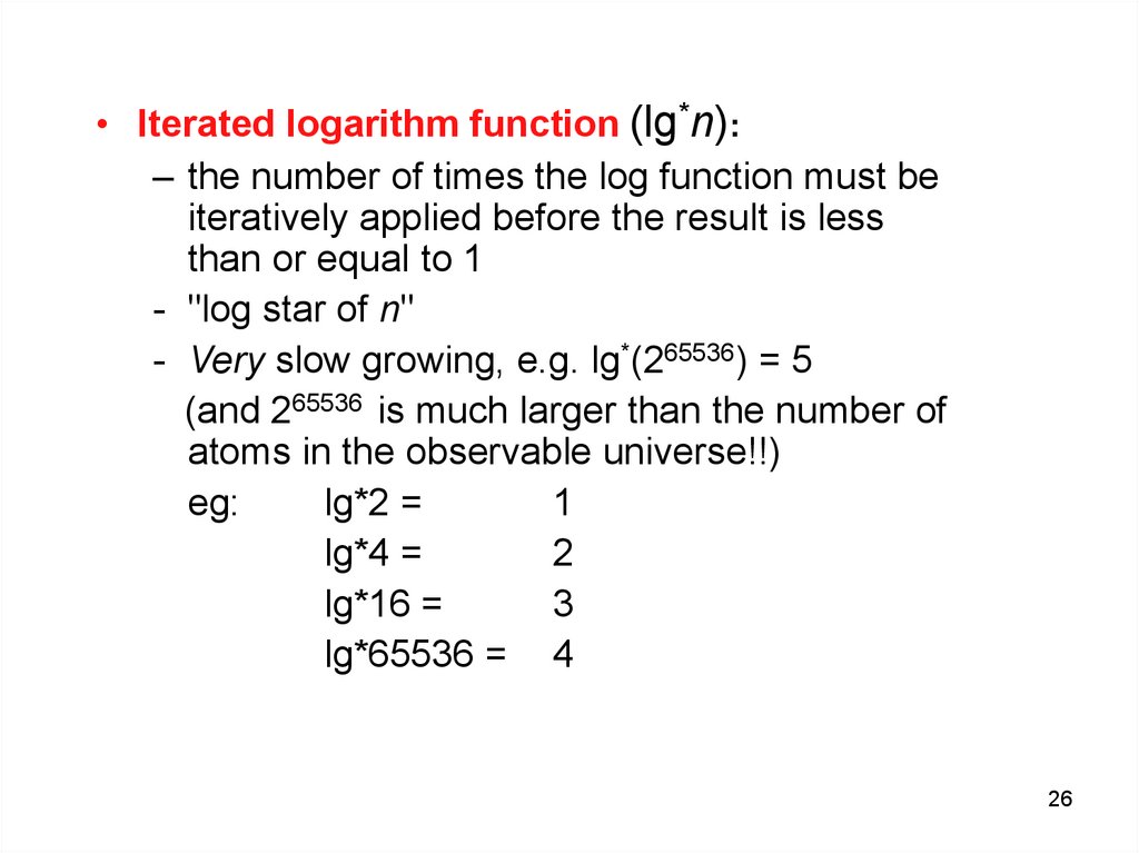
• Iterated logarithm function (lg*n):
– the number of times the log function must be
iteratively applied before the result is less
than or equal to 1
- "log star of n"
- Very slow growing, e.g. lg*(265536) = 5
(and 265536 is much larger than the number of
atoms in the observable universe!!)
eg:
lg*2 =
1
lg*4 =
2
lg*16 =
3
lg*65536 = 4
26

27.

Important Notation
Sometimes you will see
f(n) = O(n2) + O(n)
• Each occurrence of O symbol is distinct
constant.
• But O(n2) term dominates O(n) term,
equivalent to f(n) = O(n2)
27

28.

Example of O(n3)
28

29.

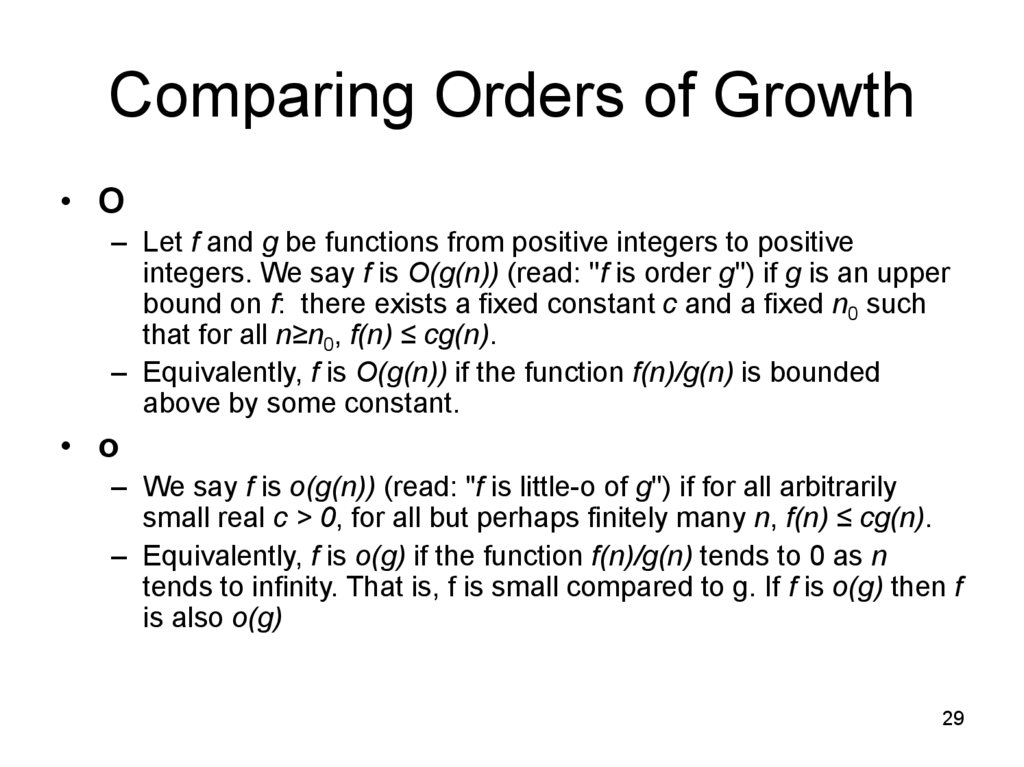
Comparing Orders of Growth
• O
– Let f and g be functions from positive integers to positive
integers. We say f is O(g(n)) (read: ''f is order g'') if g is an upper
bound on f: there exists a fixed constant c and a fixed n0 such
that for all n≥n0, f(n) ≤ cg(n).
– Equivalently, f is O(g(n)) if the function f(n)/g(n) is bounded
above by some constant.
• o
– We say f is o(g(n)) (read: "f is little-o of g'') if for all arbitrarily
small real c > 0, for all but perhaps finitely many n, f(n) ≤ cg(n).
– Equivalently, f is o(g) if the function f(n)/g(n) tends to 0 as n
tends to infinity. That is, f is small compared to g. If f is o(g) then f
is also o(g)
29

30.

• Ω
– We say that f is Ω(g(n)) (read: "f is omega of g") if g is a lower
bound on f for large n. Formally, f is Ω(g) if there is a fixed
constant c and a fixed n0 such that for all n>n0, cg(n) ≤ f(n)
– For example, any polynomial whose highest exponent is nk
is Ω(nk). If f(n) is Ω(g(n)) then g(n) is O(f(n)). If f(n) is o(g(n)) then
f(n) is not Ω(g(n)).
• Θ
– We say that f is Θ(g(n)) (read: "f is theta of g") if g is an accurate
characterization of f for large n: it can be scaled so it is both an
upper and a lower bound of f. That is, f is both O(g(n)) and
Ω(g(n)). Expanding out the definitions of Ω and O, f is Θ(g(n)) if
there are fixed constants c1 and c2 and a fixed n0 such that for all
n>n0, c1g(n) ≤ f(n) ≤ c2 g(n)
– For example, any polynomial whose highest exponent is nk
is Θ(nk). If f is Θ(g), then it is O(g) but not o(g). Sometimes
people use O(g(n)) a bit informally to mean the stronger property
Θ(g(n)); however, the two are different.
30

31.

Rules for working with orders of
growth
1. cnm = O(nk) for any constant c and any m ≤ k.
2. O(f(n)) + O(g(n)) = O(f(n) + g(n)).
3. O(f(n))O(g(n)) = O(f(n)g(n)).
4. O(cf(n)) = O(f(n)) for any constant c.
5. c is O(1) for any constant c.
6. logbn = O(log n) for any base b.
All of these rules (except #1) also hold for Q as
well.
31

32.

The simple operation with the O-notation
1. f(n)= O(f(n))
2. c O(f(n)) = O(f(n)), if c is constant
3. O(f(n))+O(g(n))= O(Max(f(n), g(n)))
3.1. O(n^2) + O(n)= ?
4. O(f(n))+O(f(n)) = ?
5. O(O(f(n)))= O(f(n))
6. O(f(n))*O(g(n))= O( (f(n)* g(n)) = f(n)*O(g(n))
6.1. O(n^2) * O(n)= ?
32

33.

The simple operation with the O-notation
1. f(n)= O(f(n))
2. c O(f(n)) = O(f(n)), if c is constant
3. O(f(n))+O(g(n))= O(Max(f(n), g(n)))
3.1. O(n^2) + O(n)= O(n^2)
4. O(f(n))+O(f(n)) = ?
5. O(O(f(n)))= O(f(n))
6. O(f(n))*O(g(n))= O( (f(n)* g(n)) = f(n)*O(g(n))
6.1. O(n^2) * O(n)= O(n^3)
33

34.

The simple operation with the O-notation
1. f(n)= O(f(n))
2. c O(f(n)) = O(f(n)), if c is constant
3. O(f(n))+O(g(n))= O(Max(f(n), g(n)))
3.1. O(n^2) + O(n)= O(n^2)
4. O(f(n))+O(f(n)) = 2 O(f(n))= O(f(n))
5. O(O(f(n)))= O(f(n))
6. O(f(n))*O(g(n))= O( (f(n)* g(n)) = f(n)*O(g(n))
6.1. O(n^2) * O(n)= ?
34

35.

The simple operation with the O-notation
1. f(n)= O(f(n))
2. c O(f(n)) = O(f(n)), if c is constant
3. O(f(n))+O(g(n))= O(Max(f(n), g(n)))
3.1. O(n^2) + O(n)= O(n^2)
4. O(f(n))+O(f(n)) = 2 O(f(n))= O(f(n))
5. O(O(f(n)))= O(f(n))
6. O(f(n))*O(g(n))= O( (f(n)* g(n)) = f(n)*O(g(n))
6.1. O(n^2) * O(n)= O(n^3)
35

36.

The simple operation with the O-notation
1. f(n)= O(f(n))
2. c O(f(n)) = O(f(n)), if c is constant
3. O(f(n))+O(g(n))= O(Max(f(n), g(n)))
3.1. O(n^2) + O(n)= O(n^2)
4. O(f(n))+O(f(n)) = 2 O(f(n))= O(f(n))
5. O(O(f(n)))= O(f(n))
6. O(f(n))*O(g(n))= O( (f(n)* g(n)) = f(n)*O(g(n))
6.1. O(n^2) * O(n)= O(n^3)
36

37.

The basic operation with the O-notation
1. f(n)= O(f(n))
2. The rule of constant c O(f(n)) = O(f(n)), if c
is constant
3. The rule for sums O(f(n))+O(g(n))=
O(Max(f(n), g(n)))
4. The rule for products
O(f(n))*O(g(n))= O( (f(n)* g(n)) = f(n)*O(g(n))
37

38.

Example 1
• O(f(n))-O(f(n))=?
38

39.

Example 1
• O(f(n))-O(f(n))=O(f(n))+ (-1)O(f(n))= ?
39

40.

Example 1
• O(f(n))-O(f(n))=O(f(n))+ (-1)O(f(n))= O(f(n))
40

41.

Example 2
Prove or disprove
O(log10 n) = O(ln n)
41

42.

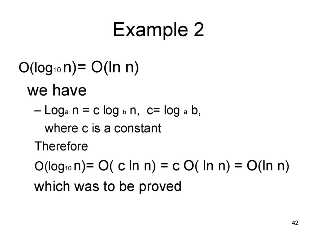
Example 2
O(log10 n)= O(ln n)
we have
– Loga n = c log b n, c= log a b,
where c is a constant
Therefore
O(log10 n)= O( c ln n) = c O( ln n) = O(ln n)
which was to be proved
42

43.

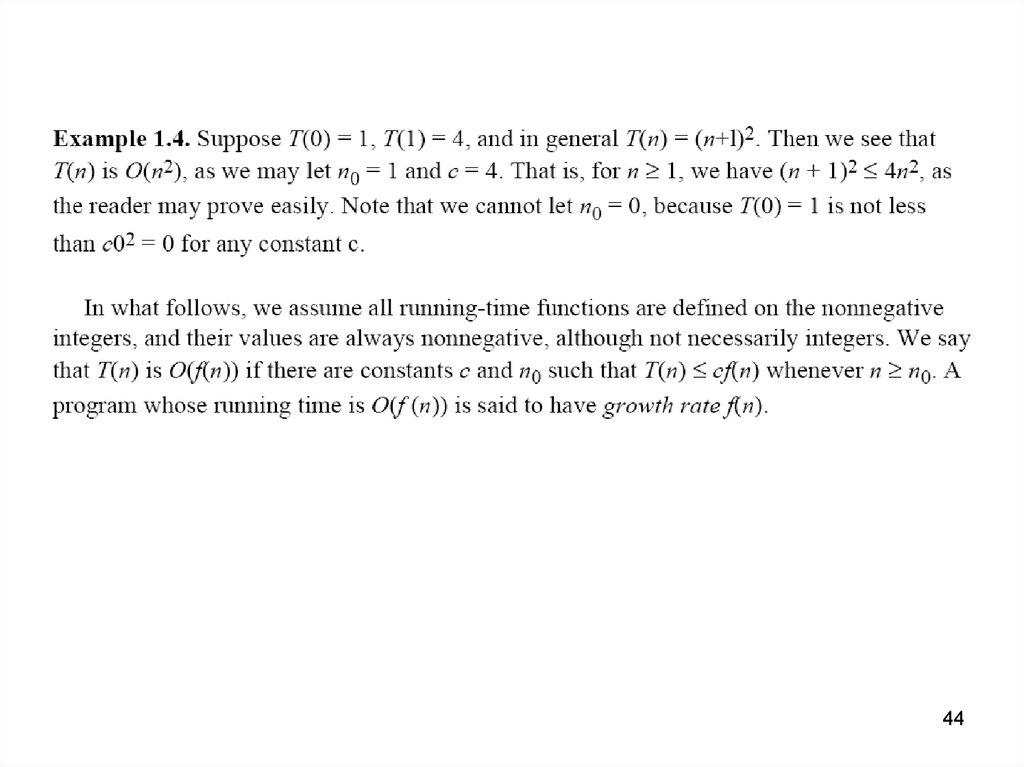
• when we say the running time T(n) of
some program is O(n^2) we mean that
there are positive constants c and n0 such
that for n equal to or greater than n0, we
have T(n) <=cn^2.
43

44.

44

45.

45

46.

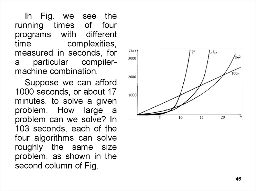
In Fig. we see the
running times of four
programs with different
time
complexities,
measured in seconds, for
a
particular
compilermachine combination.
Suppose we can afford
1000 seconds, or about 17
minutes, to solve a given
problem. How large a
problem can we solve? In
103 seconds, each of the
four algorithms can solve
roughly the same size
problem, as shown in the
second column of Fig.
46

47.

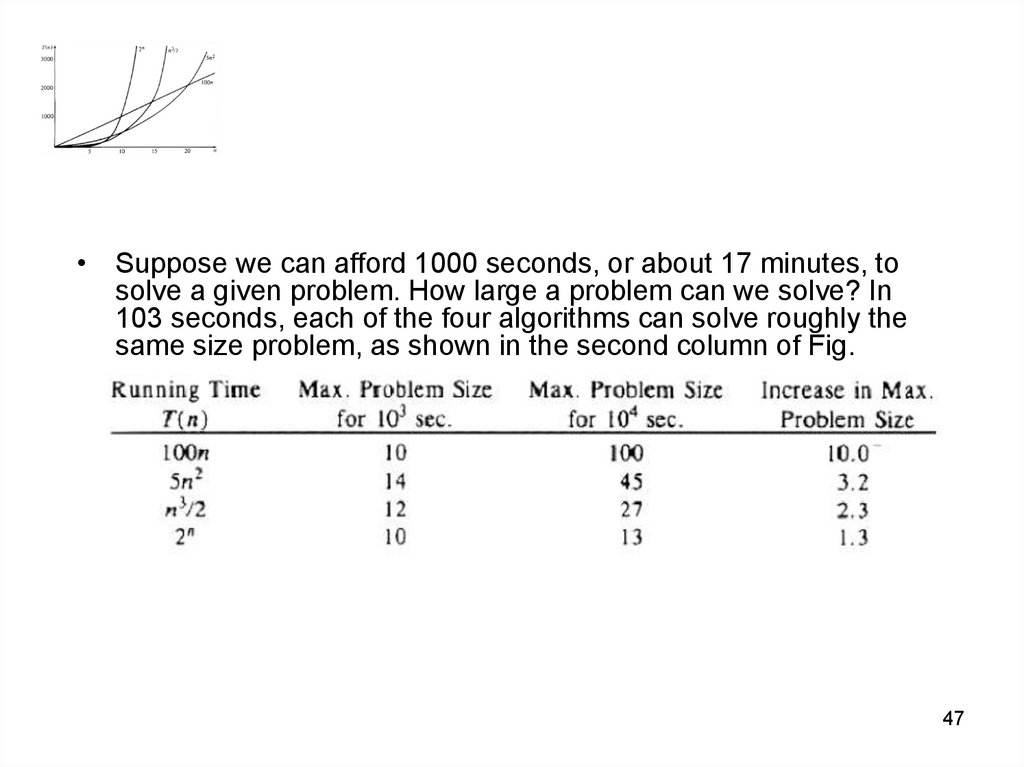
• Suppose we can afford 1000 seconds, or about 17 minutes, to
solve a given problem. How large a problem can we solve? In
103 seconds, each of the four algorithms can solve roughly the
same size problem, as shown in the second column of Fig.
47

48.

48

49.

• It is important to express logical running time in terms of physical
time, using familiar units such as seconds, minutes, hours, and
so forth to get a feel for what these characterizations really
mean. First, let's consider an O(n log(n)) algorithm that takes 1
second on an input of size 1000.
49

50.

50

51.

• The last figure greatly exceeds the age of the universe
(about 15 x 109 years), and the algorithm is already
useless at inputs of size 30. We only have acceptable
performance up to size 25 or so.
51

52.

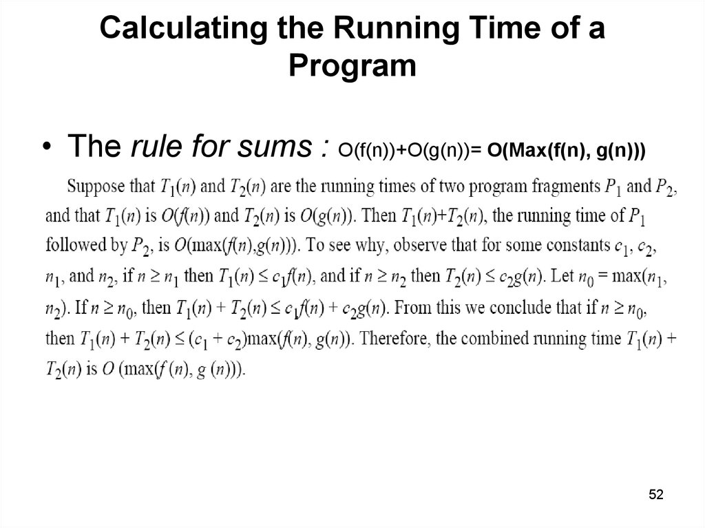
Calculating the Running Time of a
Program
• The rule for sums : O(f(n))+O(g(n))= O(Max(f(n), g(n)))
52

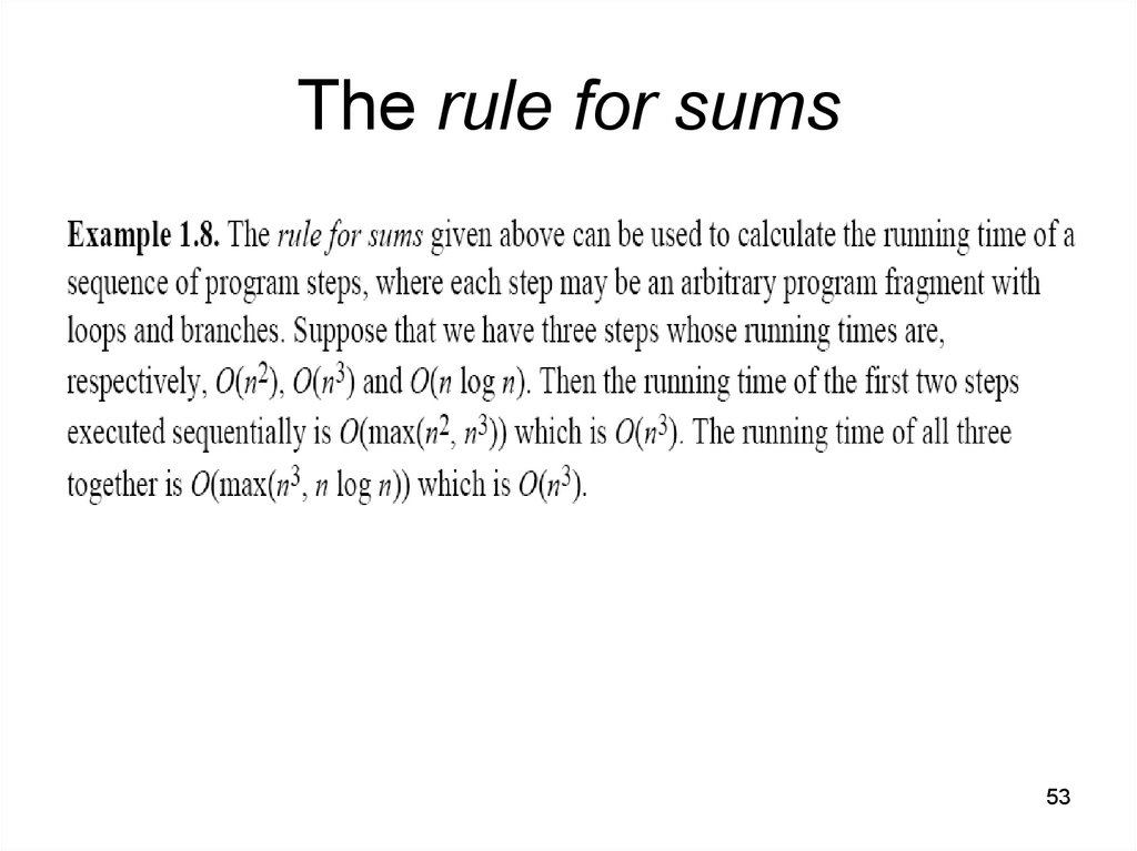
53.

The rule for sums
53

54.

The rule for products
• O(f(n))*O(g(n))= O( (f(n)* g(n))
54

55.

General rules for the analysis of
programs
1. The running time of each assignment, read, and write statement can
usually be taken to be O(1).
2. The running time of a sequence of statements is determined by the
sum rule.
3. The running time of an if-statement is the cost of the conditionally
executed statements, plus the time for evaluating the condition. The
time to evaluate the condition is normally O(1).
55

56.

Example 1
56

57.

Example 1
O(1)
O(1)
O(1)
O(1)
O(1)
O(1)
O(1)+O(1)+ O(1)+O(1)+ O(1)+ O(1) =?
57

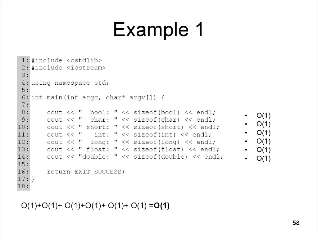
58.

Example 1
O(1)
O(1)
O(1)
O(1)
O(1)
O(1)
O(1)+O(1)+ O(1)+O(1)+ O(1)+ O(1) =O(1)
58

59.

Example 2
N*O(1), where N is argc
O(1)
O(1)
O(1)
59

60.

Example 2
N*O(1), where N is argc
O(1)
O(1)
O(1)
n*O(1)+3*O(1)=
60

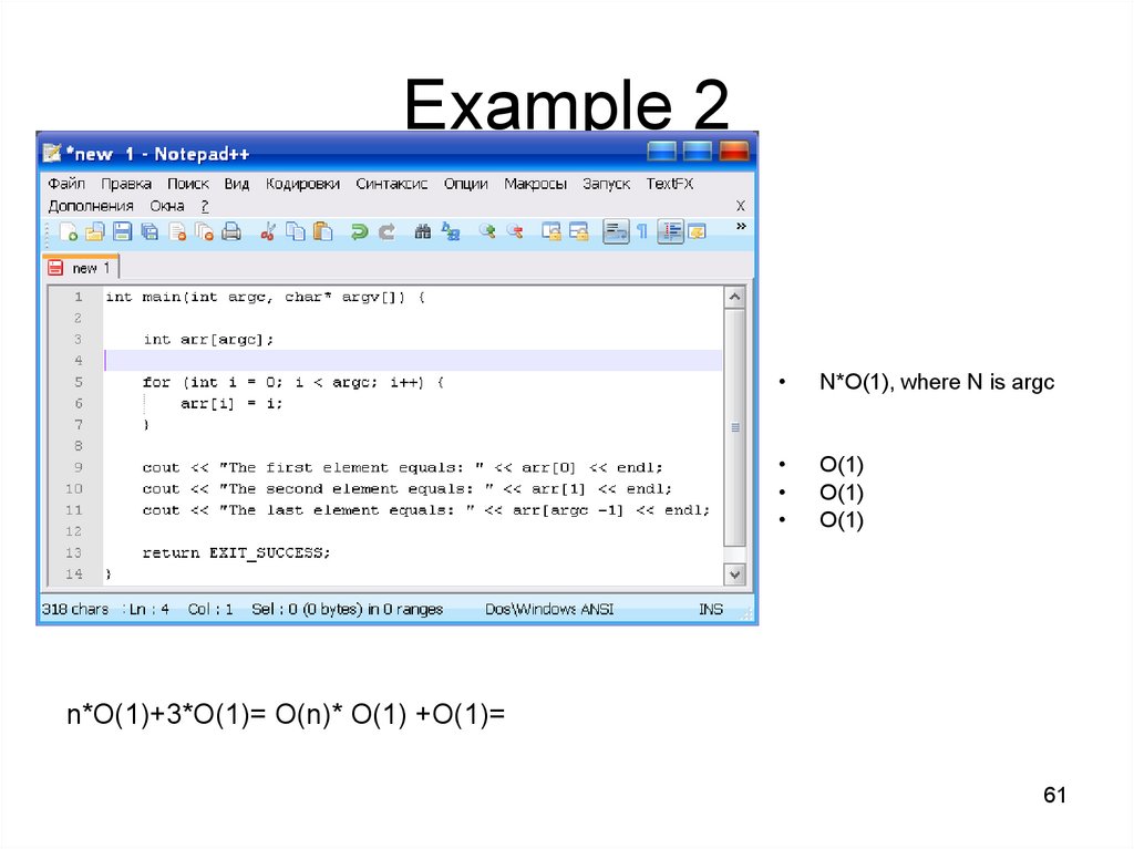
61.

Example 2
N*O(1), where N is argc
O(1)
O(1)
O(1)
n*O(1)+3*O(1)= O(n)* O(1) +O(1)=
61

62.

Example 2
N*O(1), where N is argc
O(1)
O(1)
O(1)
n*O(1)+3*O(1)= O(n)* O(1) +O(1)= O(n)
62

63.

Quiz
Consider the following C++ code fragment.
1. for( int i = 0; i < n; i++ )
2. {
3.
for( int j = 0; j < n/5; j++ ){
4.
body;
5.
}
6. }
If body executes in constant time, then the asymptotic running time that most
closely bounds from above the performance of this code fragment is
(a) O(n)
(b) O(n3)
(c) O(n2)
(d) O(n log n)
63

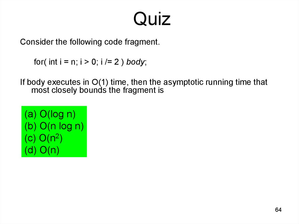
64.

Quiz
Consider the following code fragment.
for( int i = n; i > 0; i /= 2 ) body;
If body executes in O(1) time, then the asymptotic running time that
most closely bounds the fragment is
(a) O(log n)
(b) O(n log n)
(c) O(n2)
(d) O(n)
64

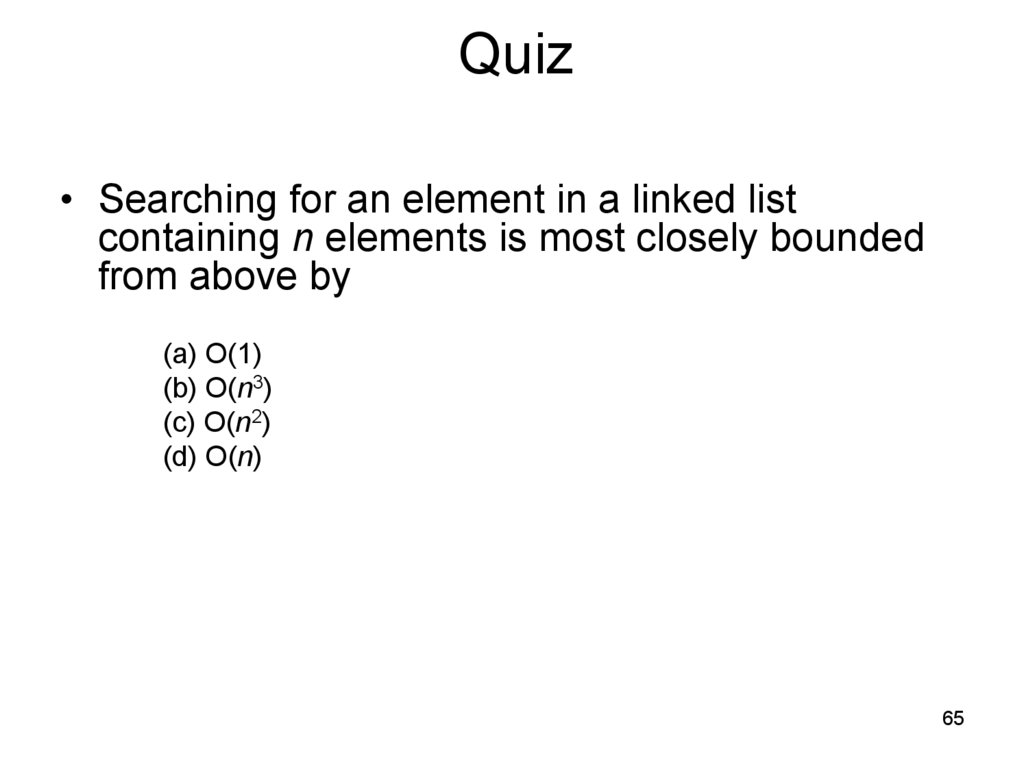
65.

Quiz
• Searching for an element in a linked list
containing n elements is most closely bounded
from above by
(a) O(1)
(b) O(n3)
(c) O(n2)
(d) O(n)
65

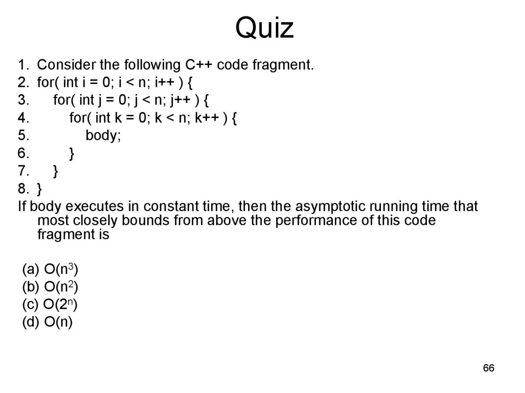
66.

Quiz
1. Consider the following C++ code fragment.
2. for( int i = 0; i < n; i++ ) {
3.
for( int j = 0; j < n; j++ ) {
4.
for( int k = 0; k < n; k++ ) {
5.
body;
6.
}
7.
}
8. }
If body executes in constant time, then the asymptotic running time that
most closely bounds from above the performance of this code
fragment is
(a) O(n3)
(b) O(n2)
(c) O(2n)
(d) O(n)
66

67.

Quiz
1. Consider the following recursive definition of a function f in C++.
2. int f(int n) {
3.
if( n == 0 ) {
4.
return 1;
5.
} else {
6.
return f(n / 2);
7.
}
8. }
The asymptotic running time of the call f(n) is most closely bound from
above by
(a) O(n2)
(b) O(log n)
(c) O(n log n)
(d) O(n)
67

68.

Reports
• Using Carrano’s book, please, prepare short report (with
presentation) about some sorting algorithms analysis.
– Selection
– Bubble
– Insertion
– Mergesort
– Quicksort
– Radix sort
– TreeSort
– etc.
• Please, prepare presentation about string sorting methods.
68

69.

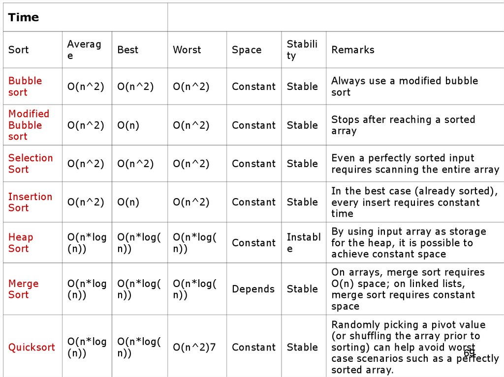
Time
Sort
Averag
e
Best
Worst
Space
Stabili
ty
Remarks
Bubble
sort
O(n^2)
O(n^2)
O(n^2)
Constant
Stable
Always use a modified bubble
sort
Modified
Bubble
sort
O(n^2)
O(n)
O(n^2)
Constant
Stable
Stops after reaching a sorted
array
Selection
Sort
O(n^2)
O(n^2)
O(n^2)
Constant
Stable
Even a perfectly sorted input
requires scanning the entire array
Constant
Stable
In the best case (already sorted),
every insert requires constant
time
Constant
Instabl
e
By using input array as storage
for the heap, it is possible to
achieve constant space
Stable
On arrays, merge sort requires
O(n) space; on linked lists,
merge sort requires constant
space
Stable
Randomly picking a pivot value
(or shuffling the array prior to
sorting) can help avoid worst
69
case scenarios such as a perfectly
sorted array.
Insertion
Sort
O(n^2)
O(n)
O(n^2)
Heap
Sort
O(n*log
(n))
O(n*log(
n))
O(n*log(
n))
Merge
Sort
Quicksort
O(n*log
(n))
O(n*log
(n))
O(n*log(
n))
O(n*log(
n))
O(n*log(
n))
O(n^2)7
Depends
Constant