 Calculating the probability of a continuous random variable – Normal Distribution")


")

 = P(z > -2) = .9772")


")


 Математика
Похожие презентации:
")
")
")
")


")


Calculating the probability of a continuous random variable – Normal Distribution. Week 9 (1)
1. BBA182 Applied Statistics Week 9 (1) Calculating the probability of a continuous random variable – Normal Distribution
DR SUSANNE HANSEN SARALEMAIL: SUSANNE.SARAL@OKAN.EDU.TR
HT TPS://PIAZZA.COM/CLASS/IXRJ5MMOX1U2T8?CID=4#
WWW.KHANACADEMY.ORG
Copyright ©2015 Pearson Education, Inc.
DR SUSANNE HANSEN SARAL
2. Mid-term exam statistics
Mid-term statisticsMean
0.563554
Median
0.57
Mode
0.61
Standard Deviation
0.173872
Sample Variance
0.030231
Kurtosis
0.080928
Skewness
-0.28804
Range
0.885
Minimum
0.115
Maximum
1
Sum
68.19
Count
121
Copyright ©2015 Pearson Education, Inc.
DR SUSANNE HANSEN SARAL
3. Mid-term exam statistics
Copyright ©2015 Pearson Education, Inc.DR SUSANNE HANSEN SARAL
4. Continuous random variable
A continuous random variable can assume any value in an intervalon the real line or in a collection of intervals.
It is not possible to talk about the probability of the random variable
assuming a particular value, because the probability will be close to
0.
Instead, we talk about the probability of the random variable
assuming a value within a given interval.
Copyright ©2015 Pearson Education, Inc.
DR SUSANNE HANSEN SARAL
5. Calculating probabilities of continuous random variables
F(b) P(X b)a
μ
b
x
a
μ
b
x
a
μ
b
x
F(a) P(X a)
P(a X b) F(b) F(a)
COPYRIGHT © 2013 PEARSON EDUCATION, INC. PUBLISHING AS PRENTICE
HALL
Ch. 5-5
6. The Standard Normal Distribution – z-values
Any normal distribution, F(x) (with any mean andstandard deviation combination) can be transformed
into the standardized normal distribution F(z), with
mean 0 and standard deviation 1
f(Z)
Z ~ N(0 ,1)
1
0
Z
We say that Z follows the standard normal distribution.
COPYRIGHT © 2013 PEARSON EDUCATION, INC. PUBLISHING AS PRENTICE
HALL
Ch. 5-6
7. Procedure for calculating the probability of x using the Standard Normal Table
For m = 100, s = 15, find the probability that X is less than 130 = P(x < 130)Transforming x - random variable into a z - standard random variable:
Z=
X -m
s
130-100
=
15
m = 100
s = 15
30
=
= 2 std dev
15
P(X < 130)
|
55
FIGURE 2.9
– Normal Distribution
Copyright ©2015 Pearson Education, Inc.
|
70
|
85
|
100
|
115
|
130
|
145
|
1
|
2
|
3
X = IQ
m
|
–3
|
–2
|
–1
DR SUSANNE HANSEN SARAL
|
0
Z=
X -m
s
8. Procedure for calculating the probability of x using the Standard Normal Table (continued)
Step 2• Look up the probability from the table of normal curve areas
• Column on the left is Z value
• Row at the top has second decimal places for Z values
Copyright ©2015 Pearson Education, Inc.
DR SUSANNE HANSEN SARAL
9. Using the Standard Normal Table
TABLE 2.10 – Standardized Normal Distribution (partial)Z
1.8
1.9
2.0
2.1
2.2
AREA UNDER THE NORMAL CURVE
0.00
0.01
0.02
0.03
0.96407
0.96485
0.96562
0.96638
0.97128
0.97193
0.97257
0.97320
0.97725
0.97784
0.97831
0.97882
0.98214
0.98257
0.98300
0.98341
0.98610
0.98645
0.98679
0.98713
For Z = 2.00
P(X < 130)
P(X > 130)
Copyright ©2015 Pearson Education, Inc.
= P(Z < 2.00) = 0.97725
= 1 – P(X ≤ 130) = 1 – P(Z ≤ 2)
= 1 – 0.97725 = 0.02275
DR SUSANNE HANSEN SARAL
10. P(z < + 2) = P(z > -2) = .9772
P(z < + 2) = P(z > -2) = .9772In probability terms, a z-score of -2.0 and +2.0 has the same probability,
because they are mirror images of each other.
If we look for the z-score 2.0 in the table we find a value of 9772.
Copyright ©2015 Pearson Education, Inc.
DR SUSANNE HANSEN SARAL
11.
The Standard Normal TableTo find the probability of: P (z > 1) and P (z < -1) we will use the
complement rule:
P( z > 1.0) = 1 - .8413 = 0.1587
.8413
.1587
0
Z
1.00
.8413
P( z < - 1.0) = 1 - .8413 = 0.1587
.1587
-1.00
Copyright ©2015 Pearson Education, Inc.
DR SUSANNE HANSEN SARAL
0
Z
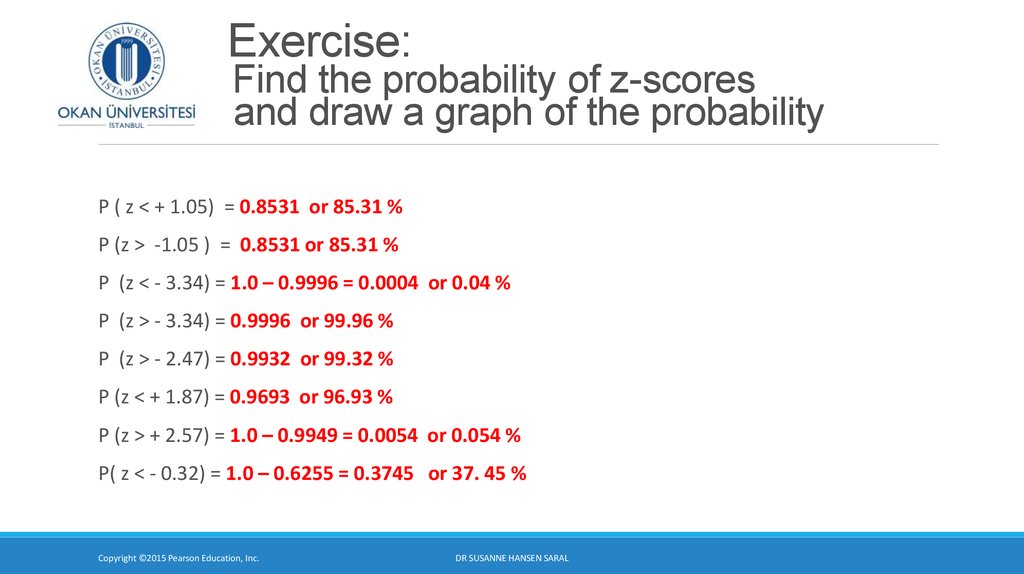
12. Finding the probability of z-scores with two decimals and graph the probability
P ( z < + 0.55) = 0.7088or 70.88 %
P (z > + .55) = 1.0 – 0.7088 = 0.2912 or 29.12%
P ( z > - 0.55) = 0.7088 or 70.88 %
P ( z < - 0.55) = 1.0 - .7088 = 0.2912 or 29.12 %
P ( z < + 1.65) = 0.9505 or 95.05 %
P (z > + 1.65) = 1.0 – 0.9505 = 0.0495 or 4.96 %
P( z > - 2.36) = .9909 or 99.09 %
P ( z < + 2.36) = .9909 or 99.09 %
Copyright ©2015 Pearson Education, Inc.
DR SUSANNE HANSEN SARAL