The Normal and other Continuous Distributions

1.

Chapter 7
The Normal and
other Continuous
Distributions
Copyright © 2017, 2015 Pearson Education. All rights reserved.
1

2.

7.1 The Standard Deviation as a Ruler
Recall that z-scores provide a standard way to compare
values.
A z-score reports the number of standard deviations
away from the mean.
In this way, we use the standard deviation as a ruler,
asking how many standard deviations a value is from the
mean.
Copyright © 2017, 2015 Pearson Education. All rights reserved.
2

3.

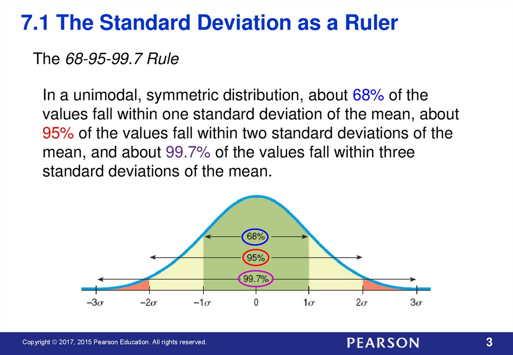
7.1 The Standard Deviation as a Ruler
The 68-95-99.7 Rule
In a unimodal, symmetric distribution, about 68% of the
values fall within one standard deviation of the mean, about
95% of the values fall within two standard deviations of the
mean, and about 99.7% of the values fall within three
standard deviations of the mean.
Copyright © 2017, 2015 Pearson Education. All rights reserved.
3

4.

7.1 The Standard Deviation as a Ruler
For Example: On August 8, 2011, the Dow dropped 634.8
points, sending shock waves through the financial
community.
During mid-2011 to mid-2012, the mean daily change for
the Dow was 1.87 with a standard deviation of 155.28
points.
The daily changes in the Dow looked unimodal and
symmetric, so use the 68-95-99.7 Rule to characterize how
extraordinary the 634.8 point drop really was.
Copyright © 2017, 2015 Pearson Education. All rights reserved.
4

5.

7.1 The Standard Deviation as a Ruler
Convert the 634.8 point drop to a z-score:
y y 634.8 1.87
z
4.10
s
155.28
A z-score with a magnitude bigger than 3 will occur with
probability of less than 0.0015, so this z-score of under 4 is
even less likely. This was a truly extraordinary event.
Copyright © 2017, 2015 Pearson Education. All rights reserved.
5

6.

7.2 The Normal Distribution
The model for symmetric, bell-shaped, unimodal histograms
is called the Normal model.
We write N(μ,σ) to represent a Normal model with mean μ
and standard deviation σ.
The model with mean 0 and standard deviation 1 is called
the standard Normal model (or the standard Normal
distribution). This model is used with standardized zscores.
Copyright © 2017, 2015 Pearson Education. All rights reserved.
6

7.

7.2 The Normal Distribution
Finding Normal Percentiles
When the standardized value falls exactly 0, 1, 2, or 3
standard deviations from the mean, we can use the 6895-99.7% rule to determine Normal probabilities.
When the standardized value does not, we can look it
up in a table of Normal percentiles.
Tables use the standard Normal model, so we’ll have to
convert our data to z-scores before using the table.
These days, we can also find probabilities associated
with z-scores use technology like calculators, statistical
software, and websites.
Copyright © 2017, 2015 Pearson Education. All rights reserved.
7

8.

7.2 The Normal Distribution
Example 1: Each Scholastic Aptitude Test (SAT) has a
distribution that is roughly unimodal and symmetric and is
designed to have an overall mean of 500 and a standard
deviation of 100.
Suppose you earned a 600 on an SAT test. From the
information above and the 68-95-99.7 Rule, where do you stand
among all students who took the SAT?
Copyright © 2017, 2015 Pearson Education. All rights reserved.
8

9.

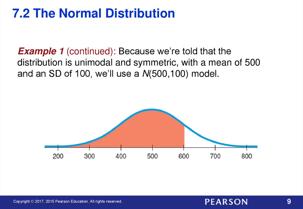
7.2 The Normal Distribution
Example 1 (continued): Because we’re told that the
distribution is unimodal and symmetric, with a mean of 500
and an SD of 100, we’ll use a N(500,100) model.
Copyright © 2017, 2015 Pearson Education. All rights reserved.
9

10.

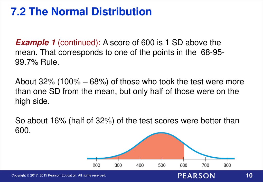
7.2 The Normal Distribution
Example 1 (continued): A score of 600 is 1 SD above the
mean. That corresponds to one of the points in the 68-9599.7% Rule.
About 32% (100% – 68%) of those who took the test were more
than one SD from the mean, but only half of those were on the
high side.
So about 16% (half of 32%) of the test scores were better than
600.
Copyright © 2017, 2015 Pearson Education. All rights reserved.
10

11.

7.2 The Normal Distribution
Example 2: Assuming the SAT scores are nearly normal
with N(500,100), what proportion of SAT scores falls
between 450 and 600?
Copyright © 2017, 2015 Pearson Education. All rights reserved.
11

12.

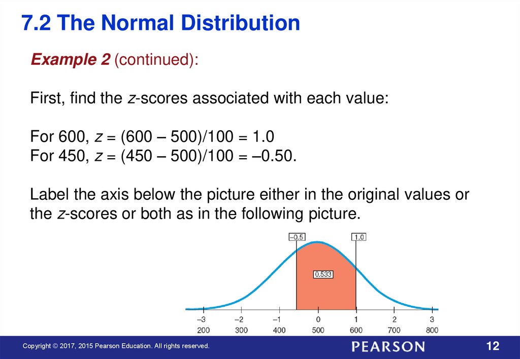
7.2 The Normal Distribution
Example 2 (continued):
First, find the z-scores associated with each value:
For 600, z = (600 – 500)/100 = 1.0
For 450, z = (450 – 500)/100 = –0.50.
Label the axis below the picture either in the original values or
the z-scores or both as in the following picture.
Copyright © 2017, 2015 Pearson Education. All rights reserved.
12

13.

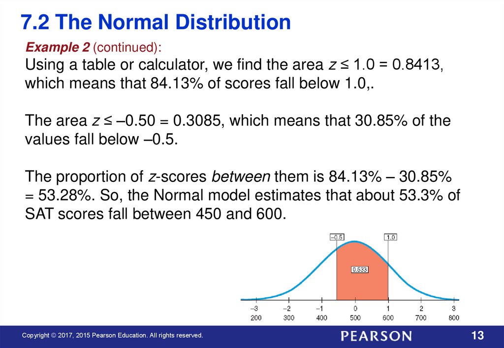
7.2 The Normal Distribution
Example 2 (continued):
Using a table or calculator, we find the area z ≤ 1.0 = 0.8413,
which means that 84.13% of scores fall below 1.0,.
The area z ≤ –0.50 = 0.3085, which means that 30.85% of the
values fall below –0.5.
The proportion of z-scores between them is 84.13% – 30.85%
= 53.28%. So, the Normal model estimates that about 53.3% of
SAT scores fall between 450 and 600.
Copyright © 2017, 2015 Pearson Education. All rights reserved.
13

14.

7.2 The Normal Distribution
Sometimes we start with areas and are asked to work
backward to find the corresponding z-score or even the
original data value.
Example 3: A college says it admits only people with SAT
scores among the top 10%. How high an SAT score does it
take to be eligible?
Copyright © 2017, 2015 Pearson Education. All rights reserved.
14

15.

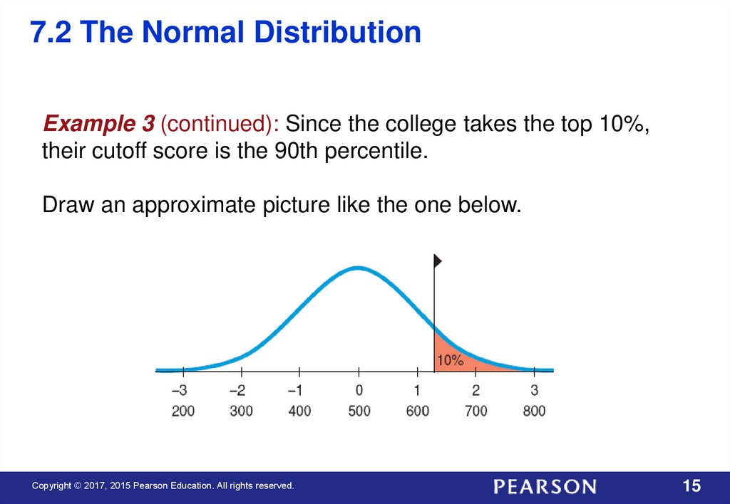
7.2 The Normal Distribution
Example 3 (continued): Since the college takes the top 10%,
their cutoff score is the 90th percentile.
Draw an approximate picture like the one below.
Copyright © 2017, 2015 Pearson Education. All rights reserved.
15

16.

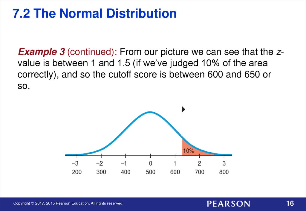
7.2 The Normal Distribution
Example 3 (continued): From our picture we can see that the zvalue is between 1 and 1.5 (if we’ve judged 10% of the area
correctly), and so the cutoff score is between 600 and 650 or
so.
Copyright © 2017, 2015 Pearson Education. All rights reserved.
16

17.

7.2 The Normal Distribution
Example 3 (continued): Using technology, you will be able to
select the 10% area and find the z-value directly.
Copyright © 2017, 2015 Pearson Education. All rights reserved.
17

18.

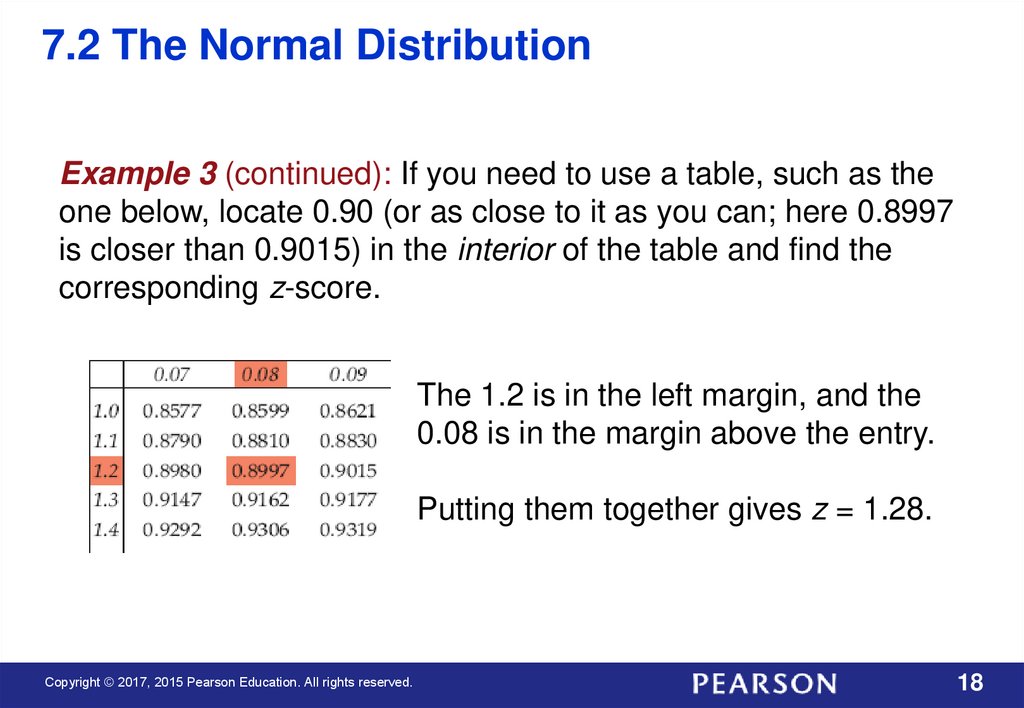
7.2 The Normal Distribution
Example 3 (continued): If you need to use a table, such as the
one below, locate 0.90 (or as close to it as you can; here 0.8997
is closer than 0.9015) in the interior of the table and find the
corresponding z-score.
The 1.2 is in the left margin, and the
0.08 is in the margin above the entry.
Putting them together gives z = 1.28.
Copyright © 2017, 2015 Pearson Education. All rights reserved.
18

19.

7.2 The Normal Distribution
Example 3 (continued): Convert the z-score back to the
original units.
A z-score of 1.28 is 1.28 standard deviations above the
mean.
Since the standard deviation is 100, that’s 128 SAT
points. The cutoff is 128 points above the mean of 500, or
628.
Since SAT scores are reported only in multiples of 10,
you’d have to score at least a 630.
Copyright © 2017, 2015 Pearson Education. All rights reserved.
19

20.

7.2 The Normal Distribution
Example: Tire Company
A tire manufacturer believes that the tread life of its snow tires
can be described by a Normal model with a mean of 32,000
miles and a standard deviation of 2500 miles.
If you buy a set of these tires, should you hope they’ll last
40,000 miles or more?
Copyright © 2017, 2015 Pearson Education. All rights reserved.
20

21.

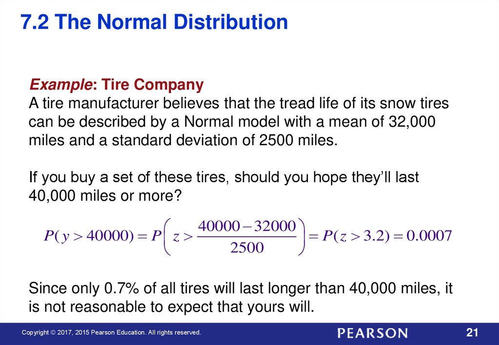
7.2 The Normal Distribution
Example: Tire Company
A tire manufacturer believes that the tread life of its snow tires
can be described by a Normal model with a mean of 32,000
miles and a standard deviation of 2500 miles.
If you buy a set of these tires, should you hope they’ll last
40,000 miles or more?
40000 32000
P( y 40000) P z
P ( z 3.2) 0.0007
2500
Since only 0.7% of all tires will last longer than 40,000 miles, it
is not reasonable to expect that yours will.
Copyright © 2017, 2015 Pearson Education. All rights reserved.
21

22.

7.2 The Normal Distribution
Example (continued): Tire Company
A tire manufacturer believes that the tread life of its snow tires
can be described by a Normal model with a mean of 32,000
miles and a standard deviation of 2500 miles.
Approximately what percent of these snow tires will last less
than 30,000 miles?
Copyright © 2017, 2015 Pearson Education. All rights reserved.
22

23.

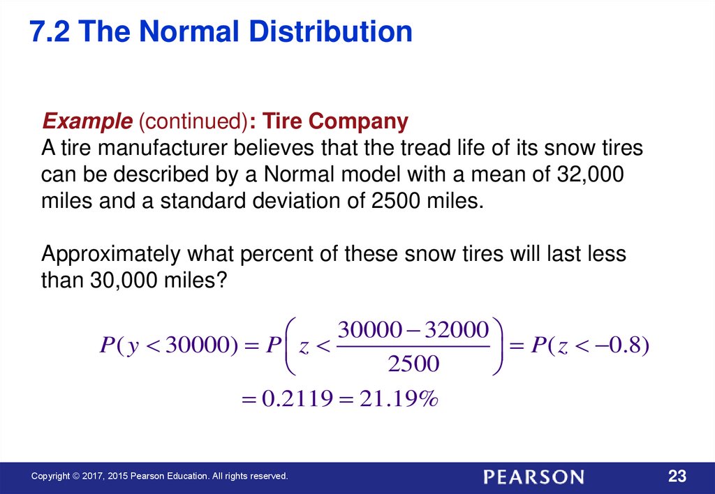
7.2 The Normal Distribution
Example (continued): Tire Company
A tire manufacturer believes that the tread life of its snow tires
can be described by a Normal model with a mean of 32,000
miles and a standard deviation of 2500 miles.
Approximately what percent of these snow tires will last less
than 30,000 miles?
30000 32000
P ( y 30000) P z
P ( z 0.8)
2500
0.2119 21.19%
Copyright © 2017, 2015 Pearson Education. All rights reserved.
23

24.

7.2 The Normal Distribution
Example (continued): Tire Company
A tire manufacturer believes that the tread life of its snow tires
can be described by a Normal model with a mean of 32,000
miles and a standard deviation of 2500 miles.
Approximately what percent of these snow tires will last
between 30,000 and 35,000 miles?
Copyright © 2017, 2015 Pearson Education. All rights reserved.
24

25.

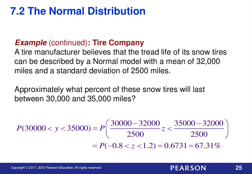
7.2 The Normal Distribution
Example (continued): Tire Company
A tire manufacturer believes that the tread life of its snow tires
can be described by a Normal model with a mean of 32,000
miles and a standard deviation of 2500 miles.
Approximately what percent of these snow tires will last
between 30,000 and 35,000 miles?
35000 32000
30000 32000
P (30000 y 35000) P
z
2500
2500
P( 0.8 z 1.2) 0.6731 67.31%
Copyright © 2017, 2015 Pearson Education. All rights reserved.
25

26.

7.2 The Normal Distribution
Example (continued): Tire Company
A tire manufacturer believes that the tread life of its snow tires
can be described by a Normal model with a mean of 32,000
miles and a standard deviation of 2500 miles.
A dealer wants to offer a refund to customers whose snow tires
fail to reach a certain number of miles, but he can only offer this
to no more than 1 out of 25 customers.
What mileage can he guarantee?
Copyright © 2017, 2015 Pearson Education. All rights reserved.
26

27.

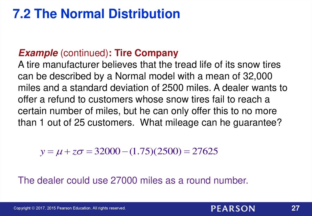
7.2 The Normal Distribution
Example (continued): Tire Company
A tire manufacturer believes that the tread life of its snow tires
can be described by a Normal model with a mean of 32,000
miles and a standard deviation of 2500 miles. A dealer wants to
offer a refund to customers whose snow tires fail to reach a
certain number of miles, but he can only offer this to no more
than 1 out of 25 customers. What mileage can he guarantee?
y z 32000 (1.75)(2500) 27625
The dealer could use 27000 miles as a round number.
Copyright © 2017, 2015 Pearson Education. All rights reserved.
27

28.

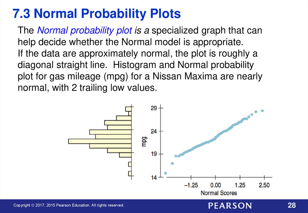
7.3 Normal Probability Plots
The Normal probability plot is a specialized graph that can
help decide whether the Normal model is appropriate.
If the data are approximately normal, the plot is roughly a
diagonal straight line. Histogram and Normal probability
plot for gas mileage (mpg) for a Nissan Maxima are nearly
normal, with 2 trailing low values.
Copyright © 2017, 2015 Pearson Education. All rights reserved.
28

29.

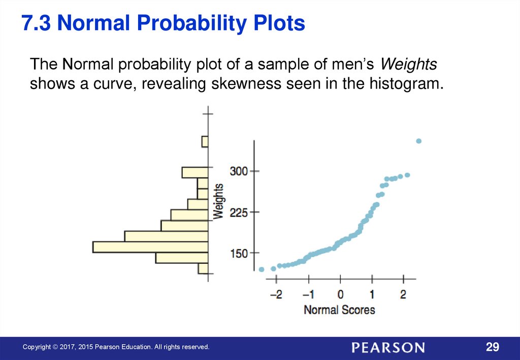
7.3 Normal Probability Plots
The Normal probability plot of a sample of men’s Weights
shows a curve, revealing skewness seen in the histogram.
Copyright © 2017, 2015 Pearson Education. All rights reserved.
29

30.

7.4 The Distribution of Sums of Normals
Normal models have many special properties. One of
these is that the sum or difference of two independent
Normal random variables is also Normal.
Copyright © 2017, 2015 Pearson Education. All rights reserved.
30

31.

7.4 The Distribution of Sums of Normals
For Example: A company that manufactures small stereo
systems uses a two-step packaging process.
Stage 1 is combining all small parts into a single packet. Then
the packet is sent to Stage 2 where it is boxed, closed, sealed
and labeled for shipping.
Stage 1 has a mean of 9 minutes and standard deviation of 1.5
minutes; Stage 2 has a mean of 6 minutes and standard
deviation of 1 minutes.
Since both stages are unimodal and symmetric, what is the
probability that packing an order of two systems takes more
than 20 minutes?
Copyright © 2017, 2015 Pearson Education. All rights reserved.
31

32.

7.4 The Distribution of Sums of Normals
Normal Model Assumption - We are told both stages are
unimodal and symmetric. And we know that the sum of two
Normal random variables is also Normal.
Independence Assumption - It is reasonable to think the
packing time for one system would not affect the packing time
for the next system.
Copyright © 2017, 2015 Pearson Education. All rights reserved.
32

33.

7.4 The Distribution of Sums of Normals
The packing stage, Stage 1, has a mean of 9 minutes and
standard deviation of 1.5 minutes.
Let
P1 = time for packing the first system
P2 = time for packing the second system
T = total time to pack two systems → T = P1 + P2
E(T) = E(P1 + P2) = E(P1 ) + E(P2) = 9 + 9 = 18 minutes
Var(P1 + P2) = Var(P1 ) + Var(P2) = 1.52 + 1.52 = 4.50
SD T 4.50 2.12 minutes
We can model the time, T, with a N(18, 2.12) model.
Copyright © 2017, 2015 Pearson Education. All rights reserved.
33

34.

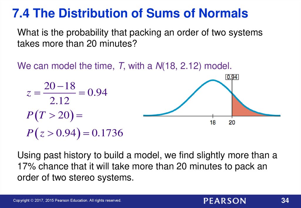
7.4 The Distribution of Sums of Normals
What is the probability that packing an order of two systems
takes more than 20 minutes?
We can model the time, T, with a N(18, 2.12) model.
20 18
z
0.94
2.12
P T 20
P z 0.94 0.1736
Using past history to build a model, we find slightly more than a
17% chance that it will take more than 20 minutes to pack an
order of two stereo systems.
Copyright © 2017, 2015 Pearson Education. All rights reserved.
34

35.

7.5 The Normal Approximation for
the Binomial
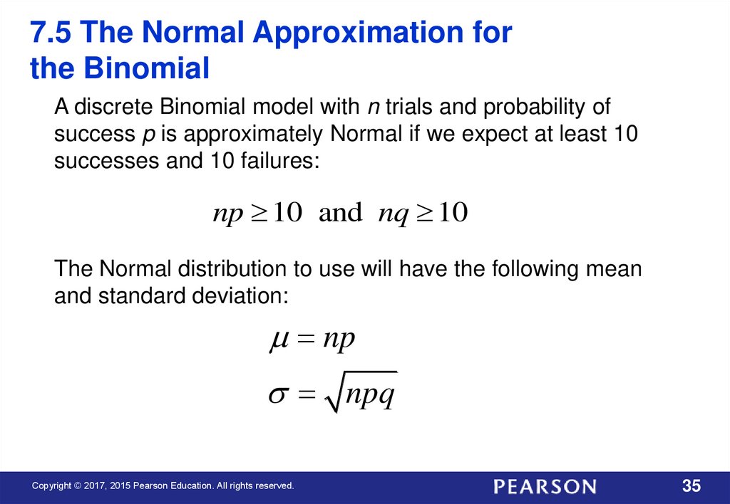
A discrete Binomial model with n trials and probability of
success p is approximately Normal if we expect at least 10
successes and 10 failures:
np 10 and nq 10
The Normal distribution to use will have the following mean
and standard deviation:
np
npq
Copyright © 2017, 2015 Pearson Education. All rights reserved.
35

36.

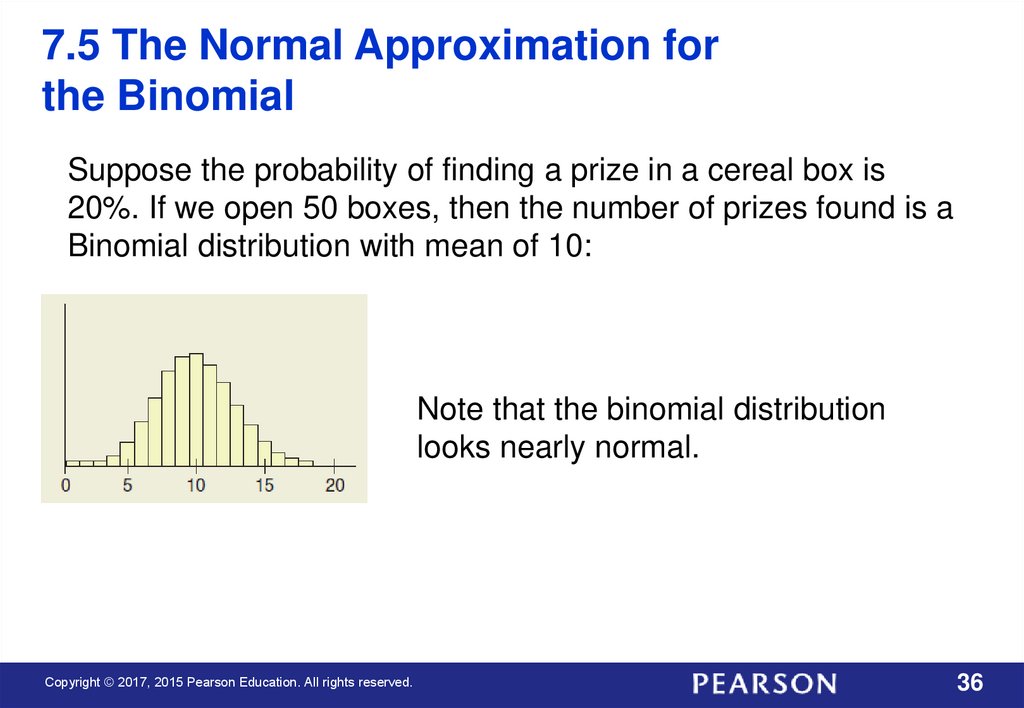
7.5 The Normal Approximation for
the Binomial
Suppose the probability of finding a prize in a cereal box is
20%. If we open 50 boxes, then the number of prizes found is a
Binomial distribution with mean of 10:
Note that the binomial distribution
looks nearly normal.
Copyright © 2017, 2015 Pearson Education. All rights reserved.
36

37.

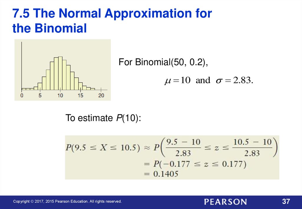
7.5 The Normal Approximation for
the Binomial
For Binomial(50, 0.2),
10 and 2.83.
To estimate P(10):
Copyright © 2017, 2015 Pearson Education. All rights reserved.
37

38.

7.6 Other Continuous Random Variables
Many phenomena in business can be modeled by
continuous random variables. The Normal model is only one
of many such models.
We will introduce just two others (entire courses are devoted
to studying which models work well in different situations):
the uniform and the exponential.
Copyright © 2017, 2015 Pearson Education. All rights reserved.
38

39.

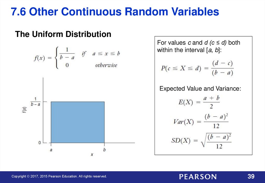
7.6 Other Continuous Random Variables
The Uniform Distribution
For values c and d (c ≤ d) both
within the interval [a, b]:
Expected Value and Variance:
Copyright © 2017, 2015 Pearson Education. All rights reserved.
39

40.

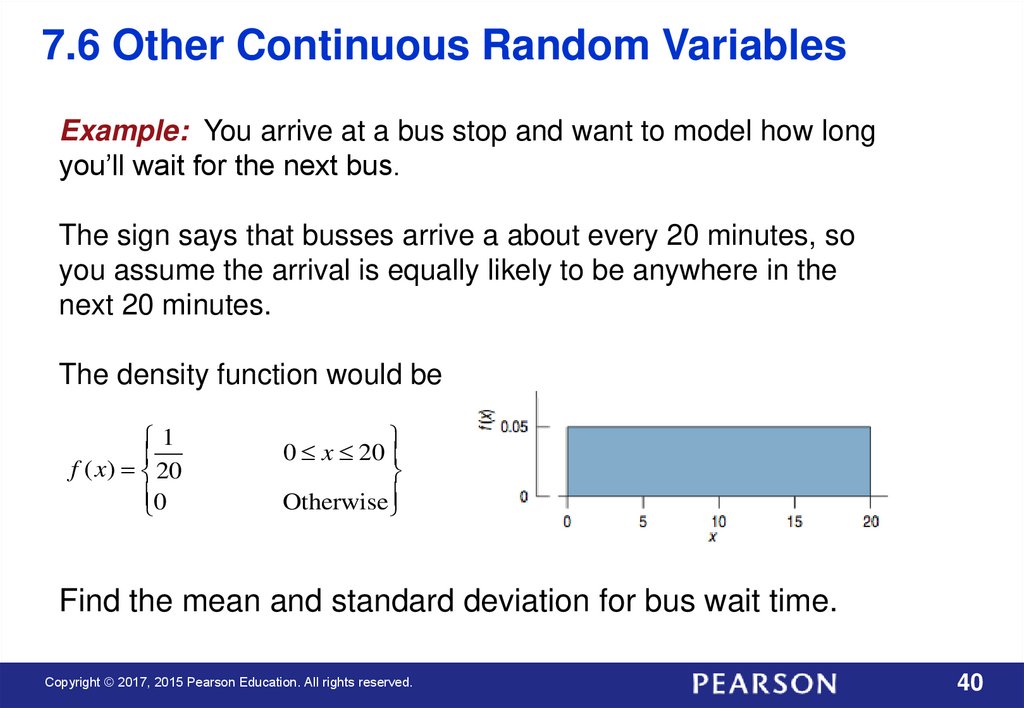
7.6 Other Continuous Random Variables
Example: You arrive at a bus stop and want to model how long
you’ll wait for the next bus.
The sign says that busses arrive a about every 20 minutes, so
you assume the arrival is equally likely to be anywhere in the
next 20 minutes.
The density function would be
1
f ( x) 20
0
0 x 20
Otherwise
Find the mean and standard deviation for bus wait time.
Copyright © 2017, 2015 Pearson Education. All rights reserved.
40

41.

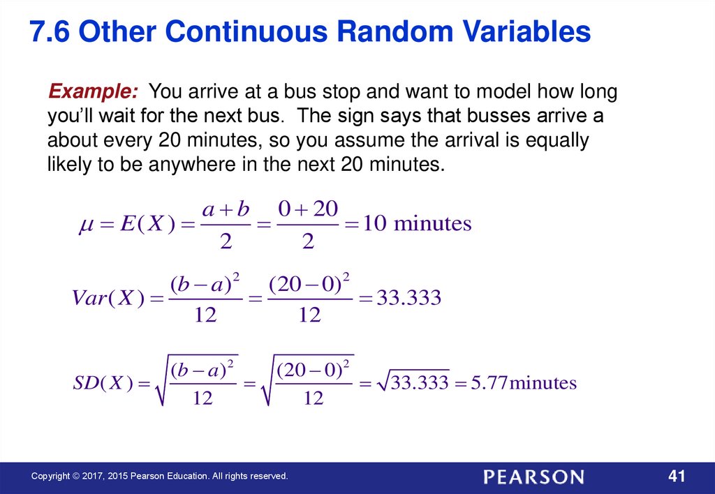
7.6 Other Continuous Random Variables
Example: You arrive at a bus stop and want to model how long
you’ll wait for the next bus. The sign says that busses arrive a
about every 20 minutes, so you assume the arrival is equally
likely to be anywhere in the next 20 minutes.
a b 0 20
E( X )
10 minutes
2
2
(b a)2 (20 0) 2
Var ( X )
33.333
12
12
SD( X )
(b a ) 2
12
(20 0) 2
33.333 5.77minutes
12
Copyright © 2017, 2015 Pearson Education. All rights reserved.
41

42.

• Probability models are still just models.
• Don’t assume everything’s Normal.
• Don’t use the Normal approximation with small n.
Copyright © 2017, 2015 Pearson Education. All rights reserved.
42

43.

What Have We Learned?
Recognize normally distributed data by making a histogram
and checking whether it is unimodal, symmetric, and bellshaped, or by making a normal probability plot using
technology and checking whether the plot is roughly a
straight line.
The Normal model is a distribution that will be important for
much of the rest of this course.
Before using a Normal model, we should check that our data
are plausibly from a Normally distributed population.
A Normal probability plot provides evidence that the data are
Normally distributed if it is linear.
Copyright © 2017, 2015 Pearson Education. All rights reserved.
43

44.

What Have We Learned?
Understand how to use the Normal model to judge whether a
value is extreme.
Standardize values to make z-scores and obtain a standard scale.
Then refer to a standard Normal distribution.
Use the 68–95–99.7 Rule as a rule-of-thumb to judge whether a
value is extreme.
Know how to refer to tables or technology to find the probability
of a value randomly selected from a Normal model falling in any
interval.
Know how to perform calculations about Normally distributed
values and probabilities.
Copyright © 2017, 2015 Pearson Education. All rights reserved.
44

45.

What Have We Learned?
Recognize when independent random Normal quantities are
being added or subtracted.
• The sum or difference will also follow a Normal model
• The variance of the sum or difference will be the sum of the
individual variances.
• The mean of the sum or difference will be the sum or difference,
respectively, of the means.
Recognize when other continuous probability distributions are
appropriate models.
Copyright © 2017, 2015 Pearson Education. All rights reserved.
45