Global-Connected Network With Generalized ReLU

1.

Global-Connected Network With Generalized ReLU Activation
Accepted Manuscript
Global-Connected Network With Generalized ReLU Activation
Zhi Chen, Pin-Han Ho
PII:
DOI:
Reference:
S0031-3203(19)30258-4
https://doi.org/10.1016/j.patcog.2019.07.006
PR 6961
To appear in:
Pattern Recognition
Received date:
Revised date:
Accepted date:
9 November 2018
9 June 2019
8 July 2019
Please cite this article as: Zhi Chen, Pin-Han Ho, Global-Connected Network With Generalized ReLU
Activation, Pattern Recognition (2019), doi: https://doi.org/10.1016/j.patcog.2019.07.006
This is a PDF file of an unedited manuscript that has been accepted for publication. As a service
to our customers we are providing this early version of the manuscript. The manuscript will undergo
copyediting, typesetting, and review of the resulting proof before it is published in its final form. Please
note that during the production process errors may be discovered which could affect the content, and
all legal disclaimers that apply to the journal pertain.
The final publication is available at Elsevier via https://doi.org/10.1016/j.patcog.2019.07.006. © 2019. This
manuscript version is made available under the CC-BY-NC-ND 4.0 license http://creativecommons.org/licenses
by-nc-nd/4.0/

2.

ACCEPTED MANUSCRIPT
1
Highlights of This Work
The contribution of this work can be summarized as follows.
1. This work presents a novel deep-connected architecture of CNN with detailed analytical analysis and
extensive experiments on several datasets.
2. A new activation function is presented to approximate arbitrary complex functions with analytical
analysis on both forward pass and backward pass.
AC
CE
PT
ED
M
AN
US
CR
IP
T
3. The experiments show the competitive performance of our designed network with less parameters and
shallower architecture, compared with other state-of-art models.
1

3.

ACCEPTED MANUSCRIPT
Zhi Chen∗, Pin-Han Ho
CR
IP
T
Global-Connected Network With Generalized ReLU
Activation
AN
US
Department of Electrical and Computer Engineering
University of Waterloo
Waterloo, Ontario, N2L 3G1, Canada
[email protected], [email protected]
Abstract
CE
PT
ED
M
Recent Progress has shown that exploitation of hidden layer neurons in convolutional neural networks (CNN) incorporating with a carefully designed activation function can yield better classification results in the field of computer
vision. The paper firstly introduces a novel deep learning (DL) architecture
aiming to mitigate the gradient-vanishing problem, in which the earlier hidden layer neurons could be directly connected with the last hidden layer and
fed into the softmax layer for classification. We then design a generalized
linear rectifier function as the activation function that can approximate arbitrary complex functions via training of the parameters. We will show that
our design can achieve similar performance in a number of object recognition
and video action benchmark tasks, such as MNIST, CIFAR-10/100, SVHN,
Fashion-MNIST, STL-10, and UCF YoutTube Action Video datasets, under
significantly less number of parameters and shallower network infrastructure,
which is not only promising in training in terms of computation burden and
memory usage, but is also applicable to low-computation, low-memory mobile scenarios for inference.
AC
Keywords: CNN, computer vision, deep learning, activation
∗
Corresponding author
Preprint submitted to Pattern Recognition
July 8, 2019

4.

ACCEPTED MANUSCRIPT
1. Introduction
AC
CE
PT
ED
M
AN
US
CR
IP
T
Deep convolution neural network (CNN) has achieved great success in
ImageNet competition [1]-[2]. In the review papers in [3]-[4], deep learning
has been well recognized as powerful tools for the computer vision applications as well as natural language processing in the recent years. This,
however, cannot be possible without the availability of massive image/video
datasets collected in the Internet-of-things era, as well as the innovation of
high-performance parallel computing resources. Exploiting these resources,
novel ideas, algorithms as well as modification on the network architecture
of deep CNN has been experimented to achieve higher performance in different computer vision tasks. Deep CNNs thus were found to be able to
extract rich hierarchical features from raw pixel values and achieved amazing performance for classification and segmentation tasks in computer vision
field.
A typical CNN usually consists of several cascaded convolution layers, optional pooling layers (average pooling, max pooling or more advanced pooling), nonlinear activations as well as fully-connected layers, followed by a
final softmax layer for classification/detection tasks, where the convolution
layer is employed to learn the spatially local-connectivity of input data for
feature extraction, pooling layer is for reduction of receptive field and hence
prohibits overfitting to some extent, and nonlinear activations for boosting of
learned features. This neural network can be learned through the well-known
backpropagation algorithm as well as momentum (for running average gradients to avoid fluctuations of stochastic gradient learning) to a very good
local optimal point, given good weight initialization and appropriate regularization. Since then, deeper CNN architecture (with more layers) [5] and
its variants, e.g., resnet [6] and highway networks [7] have been introduced
and experimented on various computer vision datasets, which are shown to
achieve state-of-the-art performance. For example, for the ImageNet challenge [1], a computer vision classification task with a massive dataset with
1000 classes of objects, the elegantly designed GoogleNet [5] achieved the
best performance on the ILSVRC 2014 competition, which employed 5 million parameters and 22 layers consisting of inception modules. This validates
the potential of deep CNN to learn powerful hierarchical information from
raw images. However, it is noted that, the advancement of deep CNN largely
follows the development of careful weight initialization, advanced regularization methods, and neural arch design. For example, to avoid overfitting
2

5.

ACCEPTED MANUSCRIPT
AC
CE
PT
ED
M
AN
US
CR
IP
T
for deep neural networks, some regularization methods are invented, such as
dropout [8][9], which turns off the neurons with a certain probability in training. By doing so, the network is forced to learn many variations of itself and
generates a natural pseudo-ensemble classifier. In [10], the authors proposed
batch normalization algorithm, providing powerful ways for co-adaptation of
features learned, which allows for higher learning rates and be less dependable on careful initialization for deep CNN. In [11], the authors considered
learning sparse representations of features from neural networks for a multitask scenario, which in some sense reduces neural network capacity whereas
avoiding overfitting to some extent.
In spite of its great success, deep CNN is subject to some open problems. One is that the features learned at an intermediate hidden layer could
be lost at classification stage. Another is the gradient vanishing problem,
which could cause training difficulty or even infeasibility. They are hence
receiving increasing interest in the literature and the industry. In this paper,
we are also motivated to mitigate such obstacles by targeting at the tasks of
real-time classification on small-scale applications. To this end, the proposed
deep CNN system incorporates a globally connected network topology with
a generalized activation function. Global average pooling (GAP) on the neurons of some hidden layers as well as the last convolution layers is applied
and results in a concatenated vector to be fed into the softmax layer. Henceforth, with only one classifier and one objective loss function for training,
we shall enjoy the benefit of retaining rich information fused in the hidden
layers while taking minimal parameters so that efficient information flow in
both forward and backward stage is guaranteed, and the overfitting risk is
avoided. Further, the proposed general activation function is composed of
several of piecewise linear functions to approximate complex functions. By
doing do, we can not only exploit the hidden layer features via rich interconnections between hidden blocks and final block, but also scales up these
learned features with the new designed activation function, leading to a more
powerful joint architecture. It will be shown in the conducted experiments
that the proposed deep CNN architecture yields similar performance with
much less parameters.
The contribution of this work is hence presented as follows.
• We present an architecture which makes full use of features learned
at hidden layers, avoiding the gradient-vanishing problem to the most
extent. The analytical analysis in closed-form on both forward pass
3

6.

ACCEPTED MANUSCRIPT
and backward pass of the proposed architecture is presented.
CR
IP
T
• We define a generalized multi-piecewise ReLU activation function, which
is able to approximate more complex and flexible functions and scales
up the learned features. The associated analytical analysis on both the
forward pass and the backward pass in closed-form is presented.
• In the conducted experiments, our design is shown to achieve promising
performance on several benchmark datasets in computer vision field,
but with less parameters and shallower structure.
M
2. Related Work
AN
US
The rest of the paper is organized as follows. In Section II some the related works are reviewed. In Section III and Section IV, the details of the
proposed deep CNN architecture as well as the designed activation function
are presented, respectively. Section V evaluates our design on several public datasets, such as MNIST [35], CIFAR-10/100 [36], SVHN [37], FashionMNIST [38], STL-10 [39], as well as UCF Youtube Action Video Data Sets
[40]. We conclude this paper in Section VI.
AC
CE
PT
ED
2.1. Activation Design
One key feature of the success of deep CNN architecture is the use of appropriate nonlinear activation functions that define the value transformation
from the input to output. It was found that the linear rectifier activation
function (ReLU) [12] can greatly boost performance of CNN in achieving
higher accuracy and faster convergence speed, in contrast to its saturated
counterpart functions, i.e., sigmoid and tanh functions. ReLU only applies
identity mapping on the positive side while drops the negative input, allowing efficient gradient propagation in training. Its simple functionality enables
training on deep neural networks without the requirement of unsupervised
pre-training and paved the way for implementations of very deep neural networks. On the other hand, one of the main drawbacks of ReLU is that
the negative part of the input is simply dropped and not updated through
backward pass, causing the problem of dead neurons which may never be reactivated again and potentially results in lost feature information through the
back-propagation. To alleviate this problem, some new types of activation
functions based on ReLU are reported for CNNs. Ng et al [13] introduced the
Leaky ReLU assigning a non-zero slope to the negative part, which however
4

7.

ACCEPTED MANUSCRIPT
AN
US
CR
IP
T
is a fixed parameter and not updated in learning. Kaiming et al pushed it
further to allow the slope on the negative side to be a learnable parameter,
which is hence named Parameter ReLU (PReLU) in [14]. Further, [15] introduced an S-shaped ReLU function. In [16], the authors introduced the ELU
activation function, which assigns an exponential function on the negative
side to zeroing the mean activation. The network performance is improved
at the cost of the increasing computation burden on the negative side, compared with other variants of ReLU. Nevertheless, all of these functions lack
the ability to mimic complex functions in order to extract necessary information relayed to the next level. In addition, Goodfellow et al introduced
a maxout function which selects the maximum among k linear functions for
each neuron as the output in [17]. While maxout has the potential to mimic
complex functions and performs well in practice, it takes much more parameters than necessary for training and thus reduces its popularity in terms of
computation and memory usage in real-time and mobile applications.
AC
CE
PT
ED
M
2.2. Network Architecture Design
The other design aspect of deep CNN is on the network size and the
interconnection mechanism of different layers. A natural way to improve
performance is to increase its size, by either depth (number of layers) or
width (number of units in each layer). This works well suited to the case
with a massive number of labelled training data. However, when the amount
of training data is small, this potentially leads to overfitting. In addition, a
non-necessary large neural net size only ends up with the waste of compute
resources, as most learned parameters may finally found to be close to zero
and can be simply dropped. Therefore, instead of changing network size,
there is an emerging trend in exploiting the interconnection of the network to
achieve better performance. The intuition follows that, the learned gradients
flowing from the output layer to the input layer, could easily be diluted or
even vanished when it reaches the beginning of the network, and vice versa.
This hence greatly prohibits performance improvement of neural networks
over decades. As discovered in the recent literature, addressing these issues
will not only allow the same performance achievable with shallower networks,
but also makes deeper networks trainable.
In [5], an inception module concatenating the feature maps produced by
filters of different sizes, i.e., a wider network consisting of many parallel convolution networks with filters of different sizes, was proposed to improve the
network capacity as well as the performance. In [6], the authors proposed
5

8.

ACCEPTED MANUSCRIPT
AC
CE
PT
ED
M
AN
US
CR
IP
T
a residual-network architecture (ResNet) to ease the training of networks,
where higher layers only need to learn a residual function with respect to
the features in the lower layers. In this way, every node only needs to learn
the residual information and thus is expected to achieve better performance
with less training time. With the residual module, the authors found that
very-deep network (e.g., a 160-layer ResNet was successfully implemented) is
trainable and can achieve amazing performance than its counterparts in the
literature. In [7], a highway network was proposed by the use of gating units
for regulating the flow of information through the network, and achieves the
state-of-art performance. In [19], a stochastic depth approach was proposed,
which only allows a subset of network modules through and replaced the
rest via identity functions in training. By doing so, it was discovered that
very-deep networks beyond 1020-layer network is trainable and achieves very
high performance. In [20], the authors proposed a neural network macroarchitecture based on self-similarity, where the designed network contains
interacting sub-paths with different lengths. In [21], a wide residual network
is proposed, which decreases depth but increases width of ResNet and also
achieves the state-of-art performance in experimentation. In [23], the hypercolumns were designed to extract useful information from intermediate
layers for segmentation and fined-grained localization at pixel level, since
the final layer information might be too coarse to locate objects. In [24], a
multi-scale spatial partition network was proposed to classify text/non-text
image classification at patch-level first for all patches from different generated feature maps from hidden layers, and then at the entire image level for
classification via voting. In [25], an end-to-end deep Fisher network, which
combines both convolution neural networks and Fisher vector encoding, was
proposed to outperform standard convolution neural networks and standard
Fisher vector methods. In [26], a weak supervision framework was proposed
to learn patch features via only image-level supervisions, and integrated multiple stages of weakly supervised object classification and discovery, achieving
state-of-art performance on benchmark datasets. In [27], a non-linear mapping with multi-layered deep neural network was employed to extract features
with mutilmodal fusion for human pose recovery. In [28], a new multiple instance neural network to learn bag representations was proposed to boost
bag classification accuracy and efficiency. In [29], a hierarchical deep neural
network with both depth and width architectures into account was proposed
for multivariate regression problems. In [30], a deep multi-task learning algorithm was developed to jointly learn features from deep convolutional neural
6

9.

ACCEPTED MANUSCRIPT
AN
US
CR
IP
T
networks and more discriminative tree classifier for automatic recommendation of privacy settings for image sharing. In [31], a deep multimodal distance
metric learning method as well as a structured ranking model were proposed
to retrieve images in a precise and efficient way.
Further, in [32], the authors introduced a Network in Network (NIN) architecture that contains several micro multi-layer perceptrons between the
convolutional layers to exploit complicated features of the input information, which is shown to reduce the number of parameters while achieve great
performance in the public datasets. In [33], the authors introduced a new
type of regularization with auxiliary classifiers employed on the hidden layers, to strengthen the features learned by hidden layers. However, the use
of the auxiliary classifiers introduces a lot of extra parameters in training,
where only the final classifier is employed in the inference stage. In [34], the
authors introduced a densely connected architecture within every block to
ensure high information flow among layers in the network, achieving stateof-art performance in most public datasets.
M
3. Global-Connected Net (GC-Net)
AC
CE
PT
ED
In this section, the proposed network architecture, namely Global-Connected
Net (GC-Net) is presented, followed by the discussion of the proposed activation function in Sec. 4.
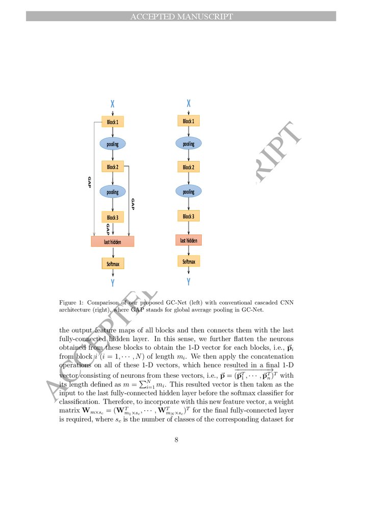
As shown in Fig. 1, the proposed GC-Net, consists of n blocks in total, a
fully-connected final hidden layer and a softmax classifier, where a block can
have several convolutional layers, each followed by normalization layers and
nonlinear activation layers. Max-pooling/Average pooling layers are applied
between connected blocks to reduce feature map sizes. The distinguished
feature of the proposed GC-Net network architecture from the conventional
cascaded structure is that, we provide a direct connection between every
block and the last hidden layer. These connections in turn create a relatively
larger vector full of rich features captured from all blocks, which is fed as
input into the last fully-connected hidden layer and then to the softmax
classifier to obtain the classification probabilities in respective of labels. In
addition, to reduce the number of parameters in use, we only allow one fullyconnected layer to the final softmax classifier, as more dense layers only has
minimal performance improvement while requires a lot of extra parameters.
In our GC-Net design, to reduce the amount of parameters as well as
computation burden, we shall first apply global average pooling (GAP) to
7

10.

GAP
X
X
Block 1
Block 1
pooling
pooling
Block 2
Block 2
pooling
pooling
AN
US
GAP
Block 3
Block 3
GAP
last hidden
ED
Y
M
last hidden
Softmax
CR
IP
T
ACCEPTED MANUSCRIPT
Softmax
Y
PT
Figure 1: Comparison of our proposed GC-Net (left) with conventional cascaded CNN
architecture (right), where GAP stands for global average pooling in GC-Net.
AC
CE
the output feature maps of all blocks and then connects them with the last
fully-connected hidden layer. In this sense, we further flatten the neurons
obtained from these blocks to obtain the 1-D vector for each blocks, i.e., ~pi
from block i (i = 1, · · · , N ) of length mi . We then apply the concatenation
operations on all of these 1-D vectors, which hence resulted in a final 1-D
−−−
−−−−−−→
T
~
vector consisting of neurons
from
these
vectors,
i.e.,
p
=
(~
p
pTn )T with
1,··· ,~
PN
its length defined as m = i=1 mi . This resulted vector is then taken as the
input to the last fully-connected hidden layer before the softmax classifier for
classification. Therefore, to incorporate with this new feature vector, a weight
T
T
matrix Wm×sc = (Wm
, · · · , Wm
)T for the final fully-connected layer
1 ×sc
N ×sc
is required, where sc is the number of classes of the corresponding dataset for
8

11.

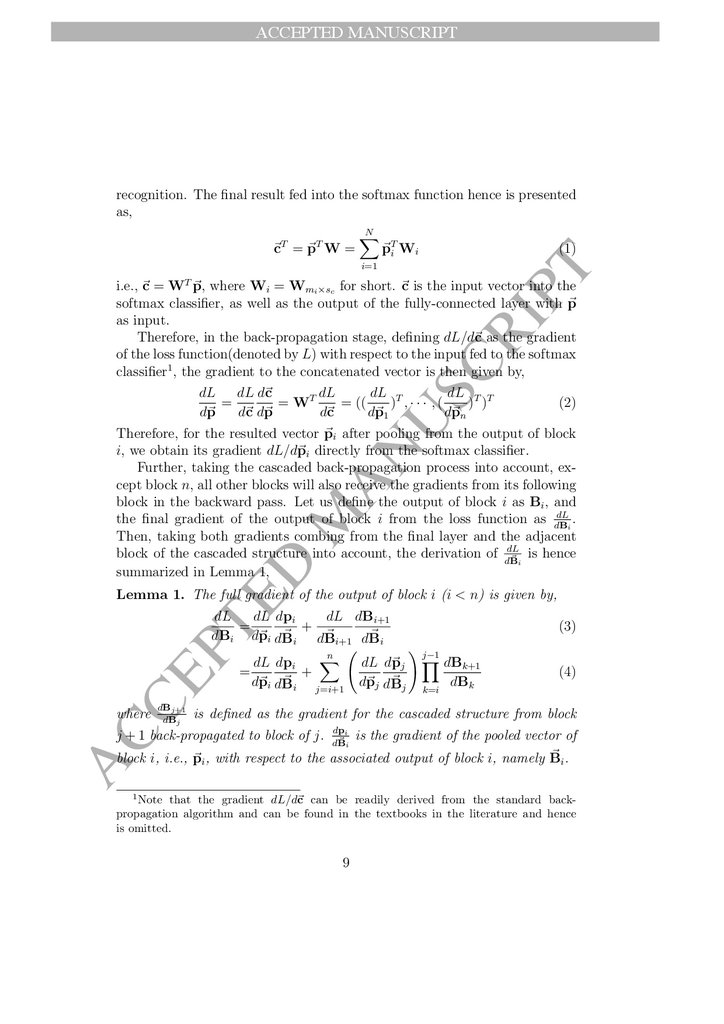
ACCEPTED MANUSCRIPT
recognition. The final result fed into the softmax function hence is presented
as,
N
X
~pTi Wi
i=1
T
(1)
CR
IP
T
~cT = ~pT W =
i.e., ~c = W ~p, where Wi = Wmi ×sc for short. ~c is the input vector into the
softmax classifier, as well as the output of the fully-connected layer with ~p
as input.
Therefore, in the back-propagation stage, defining dL/d~c as the gradient
of the loss function(denoted by L) with respect to the input fed to the softmax
classifier1 , the gradient to the concatenated vector is then given by,
ED
M
AN
US
dL d~c
dL
dL T
dL T T
dL
=
= WT
= ((
) ,··· ,(
) )
(2)
d~p
d~c d~p
d~c
d~p1
d~pn
Therefore, for the resulted vector ~pi after pooling from the output of block
i, we obtain its gradient dL/d~pi directly from the softmax classifier.
Further, taking the cascaded back-propagation process into account, except block n, all other blocks will also receive the gradients from its following
block in the backward pass. Let us define the output of block i as Bi , and
dL
.
the final gradient of the output of block i from the loss function as dB
i
Then, taking both gradients combing from the final layer and the adjacent
block of the cascaded structure into account, the derivation of ddL
~ i is hence
B
summarized in Lemma 1,
Lemma 1. The full gradient of the output of block i (i < n) is given by,
CE
PT
dL dpi
dL
dL dBi+1
=
+
~ i dB
~ i+1 dB
~i
dBi d~pi dB
where
dBj+1
dBj
n
X
dL dpi
+
=
~i
d~pi dB
j=i+1
dL d~pj
~j
d~pj dB
(3)
! j−1
Y dBk+1
k=i
dBk
(4)
is defined as the gradient for the cascaded structure from block
AC
i
j + 1 back-propagated to block of j. ddp
~ i is the gradient of the pooled vector of
B
~ i.
block i, i.e., ~pi , with respect to the associated output of block i, namely B
1
Note that the gradient dL/d~c can be readily derived from the standard backpropagation algorithm and can be found in the textbooks in the literature and hence
is omitted.
9

12.

ACCEPTED MANUSCRIPT
AC
CE
PT
ED
M
AN
US
CR
IP
T
The proof of Lemma 1 is straightforward from the chain rule in differentiation and hence is omitted. As observed in Lemma 1, each hidden block
can receive gradients from its direct connection with the last fully connected
layer. Interestingly, the earlier hidden blocks can even receive more gradients, as it not only receive the gradients directly from the last layer, backpropagated from the standard cascaded structure, but also those gradients
back-propagated from the following hidden blocks with respect to their direct
connection with the final layer. Therefore, the gradient-vanishing problem is
expected to be mitigated to some extent. In this sense, the features generated
in the hidden layer neurons are well exploited and relayed for classification.
It is noted that our design differs from all the reported research in the literature as it builds connections among blocks, instead of only within blocks,
such as ResNet [6] and Dense-connected nets [34]. Our design is also different
from the deep-supervised nets in [33] which connects every hidden layer with
an independent auxiliary classifier (and not the final layer) for regularization but the parameters with these auxiliary classifiers are not used in the
inference stage, hence results in inefficiency of parameters utilization. In our
design, in contrast to the deep-supervised net [33], each block is allowed to
connect with the last hidden layer that connects with only one final softmax
layer for classification, for both the training and inference stages. All of the
designed parameters are hence efficiently utilized to the most extent, especially in the inference stage, compared with [33]. It is noted that internal
features are also utilized in [23] and [24]. However, in [23], these features are
firstly up-sampled and summed up before fed into a tanh activation for final
classification. In [24], these intermediate-level feature maps are decomposed
into patches for classification at patch level for every patch before the final image-level classification. In our design, however, to reduce computation
burden, we do GAP on all of these feature maps and concatenate them into a
single vector for classification only at the image level with only one classifier.
Note also that by employing global average pooling (i.e., using a large kernel size for pooling) prior to the global connection in our design, the number
of resulted features from all blocks is greatly reduced, which hence significantly simplifies our structure and makes the extra number of parameters
brought by this design minimal. Further, this does not affect the depth of the
neural network, hence has negligible impact on the overall computation overhead. It is further emphasized that, in back-propagation stage, each block
can receive gradients coming from both the cascaded structure and directly
from the generated 1-D vector as well, thanks to the newly added connections
10

13.

ACCEPTED MANUSCRIPT
AN
US
CR
IP
T
between each block and the final hidden layer. Thus, the weights of the hidden layer will be better tuned, leading to higher classification performance.
It is noted that, thanks to parallel computing of GPU cores, as long as
the memory space is sufficient, the computation cost of the added features
from hidden layers on forward pass of GC-Net in Eqn. (1) is negligible. In
addition, computation overhead for the added global average pooling layers
on the hidden blocks is also minimal compared with convolution layers. For
the backward pass, it is also observed that the computation cost of GC-Net is
also minimal as we only need a split operator for gradients of pooled features
from different blocks in Eqn. (2) as well as an addition operator to sum
the hierarchical gradients and the associated GC-Net connection gradients
for specific hidden blocks in Eqn. (3). Therefore, the overall computation
overhead brought by GC-Net is minimal and can be safely neglected.
4. Generalized ReLU Activation
To collaborate with GC-Net, a new type of nonlinear activation function
is proposed and the details are presented as follows.
AC
CE
PT
ED
M
4.1. Definition and Forward Phase of GReLU
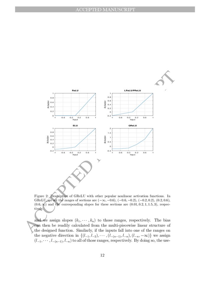
As shown in Fig. 2, the Generalized Multi-Piecewise ReLU, termed
GReLU, is defined as a combination of many piecewise linear functions as
presented in (5) as follows.
P
if x ∈ [ln , ∞);
l1 + n−1
i=1 ki (li+1 − li ) + kn (x − ln ),
.
..
if x ∈ [l1 , l2 );
l1 + k1 (x − l1 ),
x
if x ∈ [l−1 , l1 );
y(x) =
l
+
k
(x
−
l
),
if x ∈ [l−2 , l−1 );
−1
−1
−1
.
..
l + Pn−1 k (l
− l ) + k (x − l ), if x ∈ (−∞, l ).
−1
i=1
−i
−(i+1)
−i
−n
−n
−n
(5)
As defined in (5), if the inputs fall into the center range of (l−1 , l1 ), the slope
is set to be unity and the bias is set to be zero, i.e., identity mapping is
applied. Otherwise, when the inputs are larger than l1 , i.e., they fall into
one of the ranges on the positive direction in {(l1 , l2 ), · · · , (ln−1 , ln ), (ln , ∞)},
11

14.

CR
IP
T
ACCEPTED MANUSCRIPT
LReLU/PReLU
1
0.8
0.8
Activation
Activation
ReLU
1
0.6
0.4
0.2
0.4
0.2
AN
US
0
0
-0.2
-1
-0.6
-0.2
0.2
0.6
Input
1
-1
-0.6
-0.2
0.2
0.6
1
0.6
1
Input
ELU
GReLU
2
1
0.8
1.5
0.6
Activation
Activation
0.6
0.4
0.2
1
0.5
0
-0.2
-1
-0.6
-0.2
0.2
0.6
1
-0.5
-1
-0.6
-0.2
0.2
Input
PT
ED
Input
M
0
AC
CE
Figure 2: Description of GReLU with other popular nonlinear activation functions. In
GReLU, we set the ranges of sections are (−∞, −0.6), (−0.6, −0.2), (−0.2, 0.2), (0.2, 0.6),
(0.6, ∞) and the corresponding slopes for these sections are (0.01, 0.2, 1, 1.5, 3), respectively.
and we assign slopes (k1 , · · · , kn ) to those ranges, respectively. The bias
can then be readily calculated from the multi-piecewise linear structure of
the designed function. Similarly, if the inputs fall into one of the ranges on
the negative direction in {(l−1 , l−2 ), · · · , (l−(n−1) , l−n ), (l−n , −∞)} we assign
(l−1 , · · · , l−(n−1) , l−n ) to all of those ranges, respectively. By doing so, the use12

15.

ACCEPTED MANUSCRIPT
M
AN
US
CR
IP
T
ful features learned from linear mappings like convolution and fully-connected
operations are hence boosted through the designed GReLU activation function.
To fully exploit the designed multi-piecewise linear activation function,
both the endpoints li and slopes ki (i = −n, · · · , −1, 1, · · · , n) are set to
be learnable parameters, and for simplicity and computation efficiency we
restrict on channel-shared learning for the designed GReLU activation functions. Further, we do not impose constraints on the leftmost and rightmost
points, which are then learned freely while the training goes on.
Therefore, for each activation layer, GReLU only has 4n (n is the number
of ranges on both directions) learnable parameters, wherein 2n accounts for
the endpoints and another 2n for the slopes of the piecewise linear functions,
which is definitely negligible compared with millions of parameters in current
popular deep CNN models. For example, GoogleNet has 5 million parameters
and 22 layers. It is evident that, with increased n, GReLU can approximate
complex functions even better at the cost of extra computation resources
consumed, but in practice even a small n (n = 2) suffices for image/video
classification tasks.
CE
PT
ED
4.2. Relation to Other Activation Functions
It is readily observed that GReLU is a generalization of its prior counterparts. For example, setting the slopes of all sections in the positive range to
be unity (shared) and that of the sections in the negative direction another
shared slope, it degenerates into leaky ReLU if the update of parameters is
not allowed, and PReLU otherwise. Further, by setting the slopes of the
negative side to be zero, it is degenerated into ReLU function assuming no
update of parameters. In this sense, GReLU is a natural extension to these
functions, while has higher potential to learn rich features and thus perform
better than its counterparts.
AC
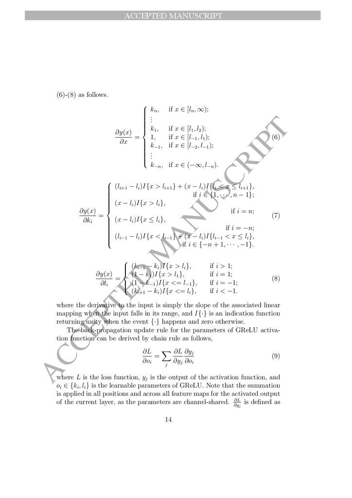
4.3. Backward Phase of GReLU
Regarding the training of GReLU, the gradient descent algorithm for
back-propagation is applied. The derivatives of the activation function with
respect to the input as well as the learnable parameters are hence given in
13

16.

ACCEPTED MANUSCRIPT
(6)-(8) as follows.
kn ,
..
.
k,
∂y(x) 1
1,
=
∂x
k−1 ,
..
.
k−n ,
if x ∈ [ln , ∞);
CR
IP
T
if x ∈ [l1 , l2 );
if x ∈ [l−1 , l1 );
if x ∈ [l−2 , l−1 );
(6)
if x ∈ (−∞, l−n ).
M
AN
US
(li+1 − li )I{x > li+1 } + (x − li )I{li < x ≤ li+1 },
if i ∈ {1, · · · , n − 1};
(x
−
l
)I{x
>
l
},
i
i
∂y(x)
if i = n;
=
(x
−
l
)I{x
≤
l
},
∂ki
i
i
if i = −n;
(l
−
l
)I{x
<
l
}
+
(x
−
l
)I{l
<
x ≤ li },
i
i−1
i
i−1
i−1
if i ∈ {−n + 1, · · · , −1}.
if i > 1;
if i = 1;
if i = −1;
if i < −1.
(8)
PT
ED
(ki−1 − ki )I{x > li },
∂y(x) (1 − k1 )I{x > l1 },
=
(1 − k−1 )I{x <= l−1 },
∂li
(ki+1 − ki )I{x <= li },
(7)
AC
CE
where the derivative to the input is simply the slope of the associated linear
mapping when the input falls in its range, and I{·} is an indication function
returning unity when the event {·} happens and zero otherwise.
The back-propagation update rule for the parameters of GReLU activation function can be derived by chain rule as follows,
∂L X ∂L ∂yj
=
∂oi
∂yj ∂oi
j
(9)
where L is the loss function, yj is the output of the activation function, and
oi ∈ {ki , li } is the learnable parameters of GReLU. Note that the summation
is applied in all positions and across all feature maps for the activated output
∂L
of the current layer, as the parameters are channel-shared. ∂y
is defined as
j
14

17.

ACCEPTED MANUSCRIPT
the derivative of the activated GReLU output back-propagated from the loss
function through its upper layers. Therefore, the simple update rule for the
learnable parameters of GReLU activation function is
∂L
∂oi
(10)
CR
IP
T
oi ← oi − α
where α is the learning rate. The weight decay (e.g., L2 regularization) is
not taken into account in updating these parameters.
M
AN
US
4.4. Benefits of GReLU
From the discussion above, it is therefore found out that designing GReLU
as a multi-piecewise linear function has several benefits, compared to its
counterparts. One is that it enables approximation of complex functions
whether they are convex functions or not, while most of activation functions
however cannot. This demonstrates its stronger capability in feature learning.
Further, since it only employs linear mappings in different ranges along the
dimension, it inherits the advantage of the non-saturate functions, i.e., the
gradient vanishing/exploding effect is mitigated to the most extent. We shall
discuss its effect further in the experiment part.
AC
CE
PT
ED
4.5. Computation Complexity Analysis
Due to the fact that we have 2n learnable parameters for slopes and 2n
learnable parameters for sections, it is observed from forward pass in Eqn.
(5), at most O(log (2n + 1)) time complexity is required to find the right
interval for data points, while the computation cost of the linear operator
(e.g., y = a+b(x−x0 )) is kind of complexity O(1) and is minimal. Regarding
the backward pass in Eqn. (6)-(8), the computation cost is also bounded
up by O(log (2n + 1)) in Eqn. (6) while O(2) in Eqn. (7) (at most two
comparison operators in indication functions) and O(1) in Eqn. (8) with only
one comparison operator. In this sense, the computation cost of one GReLU
activation is of the order of O(log (2n + 1)) ReLU activation functions, and
is negligible with small n, as the computation cost of ReLU activations in
neural networks is minimal compared with other layers in neural models.
5. Experiments and Analysis
5.1. Overall Setting
The following public datasets with different scales, MNIST, CIFAR10, CIFAR100, Fashion-MNIST, SVHN, and UCF YouTube Action Video datasets,
15

18.

ACCEPTED MANUSCRIPT
AN
US
CR
IP
T
are employed to test the proposed GC-Net and GReLU. Experiments are
firstly conducted on small neural nets using the small dataset MNIST and
compare the resultant performance with that by the traditional CNN schemes.
Then we move to a larger CNN for performance comparison with other stateof-the-art models, such as stochastic pooling, NIN [32] and Maxout [17], for
all of these datasets. Due to the complexity of GReLU, we freeze the learning of slopes and endpoints in the first few steps treating it like a Leaky
ReLU function, and then starts to learn them thereafter. Our experiments
are implemented in PYTORCH with one Nvidia GeForce GTX 1080 and we
use ADAM optimizer to update weights for the experiments if not otherwise
noted. It is also noted that in all experiments we do not apply data augmentation on these considered datasets2 Better results are hence expected with
extensive search for these parameters..
AC
CE
PT
ED
M
5.2. MNIST On SmallNet
The MNIST digit dataset [35] contains 70000 28 × 28 gray-scale images
of numerical digits from 0 to 9. The dataset is divided into the training set
with 60000 images and the test set with 10000 images.
In this SmallNet experiment, MNIST is used for performance comparison
between our model with conventional ones, as well as study on effects of both
the GC-Net as well as the new designed activation function. The proposed
GReLU activated GC-Net (GC-Net-GReLU) is composed of 3 convolution
layers with small 3×3 filters and only 16, 16 and 32 feature maps, respectively.
The 2×2 max pooling layer with a stride of 2×2 was applied after both of the
first two convolution layers. GAP is applied to the output of each convolution
layer and the collected averaged features are fed as input to the softmax
layer for classification. The total number of parameters amounts to be only
around 8.3K. For a fair comparison, we also examined the dataset using a
3-convolution-layer CNN with ReLU activation (C-CNN-ReLU), with 16, 16
and 36 feature maps equipped in the three convolutional layers, respectively.
Therefore, both tested networks use a similar amount of parameters (if not
the same).
In MNIST, neither preprocessing nor data augmentation was performed
on this dataset, except we re-scale the pixel values to be within (−1, 1) range.
2
The hyperparameters used in all the experiments are only manually set due to the
computation resources constraint while the slopes and end-points of GReLU are manually
initialized.
16

19.

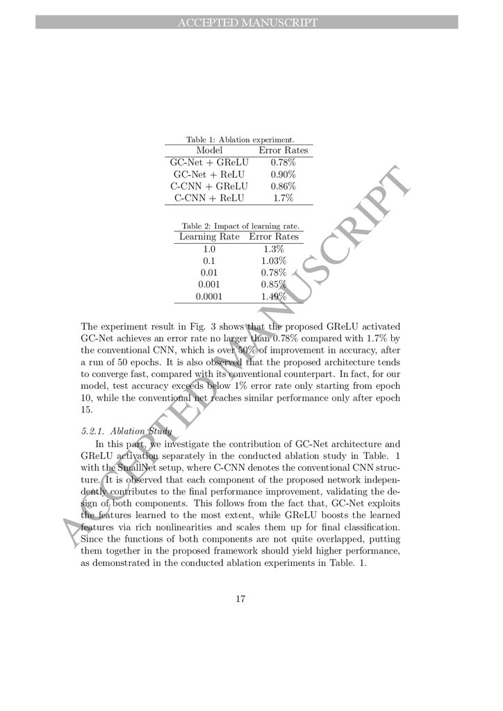
ACCEPTED MANUSCRIPT
Table 1: Ablation experiment.
Error Rates
0.78%
0.90%
0.86%
1.7%
Table 2: Impact of learning rate.
Error Rates
1.3%
1.03%
0.78%
0.85%
1.49%
AN
US
Learning Rate
1.0
0.1
0.01
0.001
0.0001
CR
IP
T
Model
GC-Net + GReLU
GC-Net + ReLU
C-CNN + GReLU
C-CNN + ReLU
ED
M
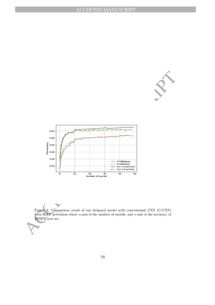
The experiment result in Fig. 3 shows that the proposed GReLU activated
GC-Net achieves an error rate no larger than 0.78% compared with 1.7% by
the conventional CNN, which is over 50% of improvement in accuracy, after
a run of 50 epochs. It is also observed that the proposed architecture tends
to converge fast, compared with its conventional counterpart. In fact, for our
model, test accuracy exceeds below 1% error rate only starting from epoch
10, while the conventional net reaches similar performance only after epoch
15.
AC
CE
PT
5.2.1. Ablation Study
In this part, we investigate the contribution of GC-Net architecture and
GReLU activation separately in the conducted ablation study in Table. 1
with the SmallNet setup, where C-CNN denotes the conventional CNN structure. It is observed that each component of the proposed network independently contributes to the final performance improvement, validating the design of both components. This follows from the fact that, GC-Net exploits
the features learned to the most extent, while GReLU boosts the learned
features via rich nonlinearities and scales them up for final classification.
Since the functions of both components are not quite overlapped, putting
them together in the proposed framework should yield higher performance,
as demonstrated in the conducted ablation experiments in Table. 1.
17

20.

CE
PT
ED
M
AN
US
CR
IP
T
ACCEPTED MANUSCRIPT
AC
Figure 3: Comparison result of our designed model with conventional CNN (C-CNN)
with ReLU activation where x-axis is the number of epochs, and y-axis is the accuracy of
MNIST test set.
18

21.

ACCEPTED MANUSCRIPT
Table 3: Error rates on MNIST without data augmentation.
Error Rates
0.47%
0.47%
0.51%
0.39%
0.47%
0.35%
0.42%
0.27%
CR
IP
T
No. of Param.(MB)
0.22M
0.42M
0.35M
0.35M
0.35M
0.35M + 5.68K
0.078M
0.22M
AN
US
Model
Stochastic Pooling
Maxout
DSN+softmax
DSN+SVM
NIN + ReLU
NIN + SReLU
GReLU-GC-Net
GReLU-GC-Net
ED
M
5.2.2. Impact of Learning Rate
In this part, we discuss the impact of some optimizer hyperparameter, i.e.,
specifically the learning rate. We hence conducted experiments on GC-Net
with GReLU by applying different learning rates as shown in Table. 2 with
the SmallNet setup. As expected, learning rate of 1.0 is kind of too large and
cannot reach 1% error rate. Instead, a learning rate of 0.01 is good enough
to achieve the highest performance, since MNIST is a simple classification
task. With the learning rate as small as 0.0001, the network weights might
not be sufficiently updated or probably get stuck at some saddle points, and
hence the performance is the worst.
AC
CE
PT
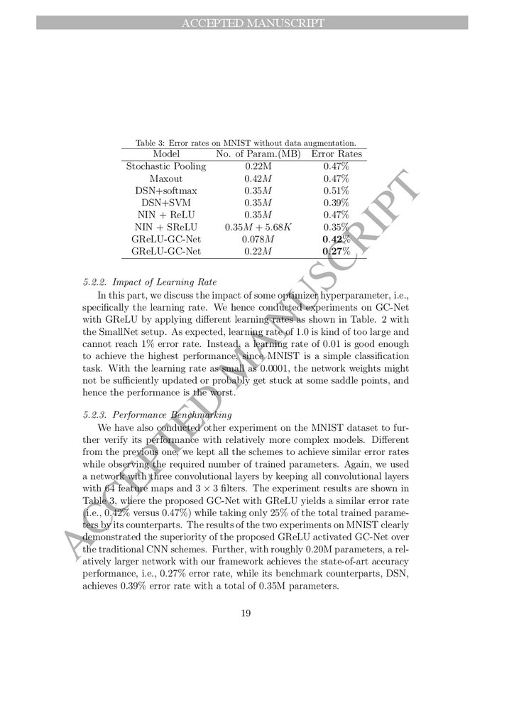
5.2.3. Performance Benchmarking
We have also conducted other experiment on the MNIST dataset to further verify its performance with relatively more complex models. Different
from the previous one, we kept all the schemes to achieve similar error rates
while observing the required number of trained parameters. Again, we used
a network with three convolutional layers by keeping all convolutional layers
with 64 feature maps and 3 × 3 filters. The experiment results are shown in
Table 3, where the proposed GC-Net with GReLU yields a similar error rate
(i.e., 0.42% versus 0.47%) while taking only 25% of the total trained parameters by its counterparts. The results of the two experiments on MNIST clearly
demonstrated the superiority of the proposed GReLU activated GC-Net over
the traditional CNN schemes. Further, with roughly 0.20M parameters, a relatively larger network with our framework achieves the state-of-art accuracy
performance, i.e., 0.27% error rate, while its benchmark counterparts, DSN,
achieves 0.39% error rate with a total of 0.35M parameters.
19

22.

ACCEPTED MANUSCRIPT
PT
ED
M
AN
US
CR
IP
T
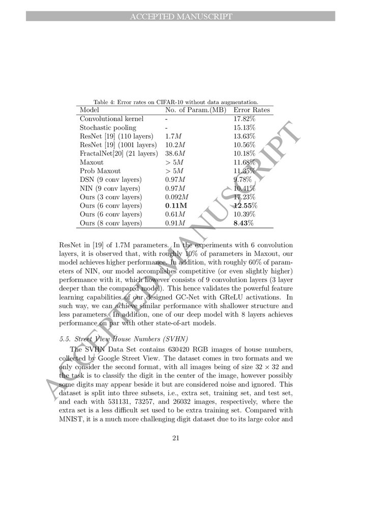
5.3. CIFAR10
The CIFAR-10 dataset contains 60000 natural color (RGB) images with
a size of 32 × 32 in 10 general object classes. The dataset is divided into
50000 training images and 10000 testing images. All of our experiments are
implemented without data augmentation and we employ the same preprocessing strategy in [32]. The comparison results of the proposed GReLU
activated GC-Net to the reported methods in the literature on this dataset,
including stochastic pooling, maxout [17], NIN [32], are given in Table. 4.
It is observed that our method achieves comparable performance while taking greatly reduced number of parameters employed in other models. Interestingly, one of our shallow model with only 0.092M parameters in 3
convolution layers achieves comparable performance with convolution kernel
method. For the experiments with 6 convolution layers and only 0.11M parameters, our model achieves promising performance with error rate around
12.6%. With roughly 0.61M parameters, our model achieves comparable performance in contrast to Maxout with 5M parameters. Actually, compared
with NIN consisting of 9 convolution layers and roughly 1M parameters,
our model achieves competitive performance, only in a 6-convolution-layer
shallow architecture with roughly 60% of parameters of it. These results
hence well demonstrate the advantage of our proposed GReLU activated
GC-Net method, which accomplishes similar performance with less parameters and a shallower structure (less convolution layers required), and hence
is appropriate for memory-efficient and computation-efficient scenarios, such
as mobile/embedded applications. In addition, it is observed that, our 9convolution-layer model is able to achieve around 8.4% error rate with only
around 1M parameters without data augmentation.
AC
CE
5.4. CIFAR100
The CIFAR-100 dataset also contain 60000 natural color (RGB) images
with a size of 32×32 but in 100 general object classes. The dataset is divided
into 50000 training images and 10000 testing images. Our experiments on
this dataset are implemented without data augmentation and we employ
the same preprocessing strategy in [32]. The comparison results of our model
to the reported methods in the literature on this dataset, are given in Table.
5. It is observed that our method achieves comparable performance while
taking greatly reduced number of parameters employed in other models. As
observed in Table. 5, one of our shallow model with only 0.16M parameters and 3 convolution layers, achieves comparable performance with deep
20

23.

ACCEPTED MANUSCRIPT
Table 4: Error rates on CIFAR-10 without data augmentation.
AN
US
CR
IP
T
Model
No. of Param.(MB) Error Rates
Convolutional kernel
17.82%
Stochastic pooling
15.13%
ResNet [19] (110 layers)
1.7M
13.63%
ResNet [19] (1001 layers) 10.2M
10.56%
FractalNet[20] (21 layers) 38.6M
10.18%
Maxout
> 5M
11.68%
Prob Maxout
> 5M
11.35%
DSN (9 conv layers)
0.97M
9.78%
NIN (9 conv layers)
0.97M
10.41%
Ours (3 conv layers)
0.092M
17.23%
Ours (6 conv layers)
0.11M
12.55%
Ours (6 conv layers)
0.61M
10.39%
Ours (8 conv layers)
0.91M
8.43%
PT
ED
M
ResNet in [19] of 1.7M parameters. In the experiments with 6 convolution
layers, it is observed that, with roughly 10% of parameters in Maxout, our
model achieves higher performance. In addition, with roughly 60% of parameters of NIN, our model accomplishes competitive (or even slightly higher)
performance with it, which however consists of 9 convolution layers (3 layer
deeper than the compared model). This hence validates the powerful feature
learning capabilities of our designed GC-Net with GReLU activations. In
such way, we can achieve similar performance with shallower structure and
less parameters. In addition, one of our deep model with 8 layers achieves
performance on par with other state-of-art models.
AC
CE
5.5. Street View House Numbers (SVHN)
The SVHN Data Set contains 630420 RGB images of house numbers,
collected by Google Street View. The dataset comes in two formats and we
only consider the second format, with all images being of size 32 × 32 and
the task is to classify the digit in the center of the image, however possibly
some digits may appear beside it but are considered noise and ignored. This
dataset is split into three subsets, i.e., extra set, training set, and test set,
and each with 531131, 73257, and 26032 images, respectively, where the
extra set is a less difficult set used to be extra training set. Compared with
MNIST, it is a much more challenging digit dataset due to its large color and
21

24.

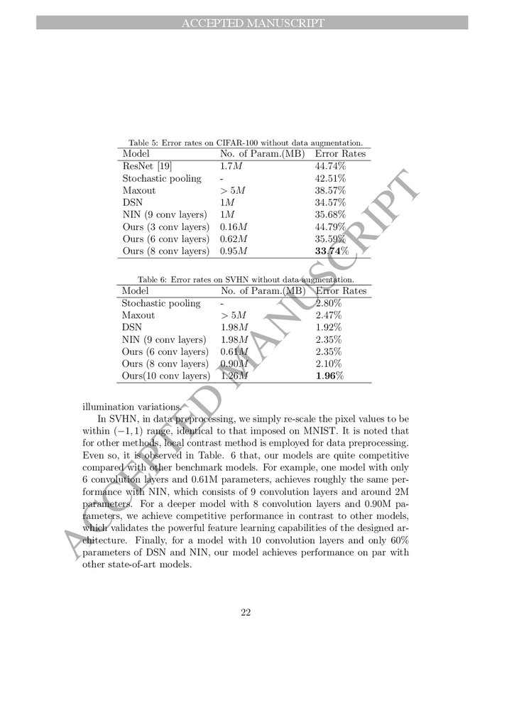
ACCEPTED MANUSCRIPT
Table 5: Error rates on CIFAR-100 without data augmentation.
No. of Param.(MB) Error Rates
1.7M
44.74%
42.51%
> 5M
38.57%
1M
34.57%
1M
35.68%
0.16M
44.79%
0.62M
35.59%
0.95M
33.74%
CR
IP
T
Model
ResNet [19]
Stochastic pooling
Maxout
DSN
NIN (9 conv layers)
Ours (3 conv layers)
Ours (6 conv layers)
Ours (8 conv layers)
No. of Param.(MB)
> 5M
1.98M
1.98M
0.61M
0.90M
1.26M
ED
M
Model
Stochastic pooling
Maxout
DSN
NIN (9 conv layers)
Ours (6 conv layers)
Ours (8 conv layers)
Ours(10 conv layers)
AN
US
Table 6: Error rates on SVHN without data augmentation.
Error Rates
2.80%
2.47%
1.92%
2.35%
2.35%
2.10%
1.96%
AC
CE
PT
illumination variations.
In SVHN, in data preprocessing, we simply re-scale the pixel values to be
within (−1, 1) range, identical to that imposed on MNIST. It is noted that
for other methods, local contrast method is employed for data preprocessing.
Even so, it is observed in Table. 6 that, our models are quite competitive
compared with other benchmark models. For example, one model with only
6 convolution layers and 0.61M parameters, achieves roughly the same performance with NIN, which consists of 9 convolution layers and around 2M
parameters. For a deeper model with 8 convolution layers and 0.90M parameters, we achieve competitive performance in contrast to other models,
which validates the powerful feature learning capabilities of the designed architecture. Finally, for a model with 10 convolution layers and only 60%
parameters of DSN and NIN, our model achieves performance on par with
other state-of-art models.
22

25.

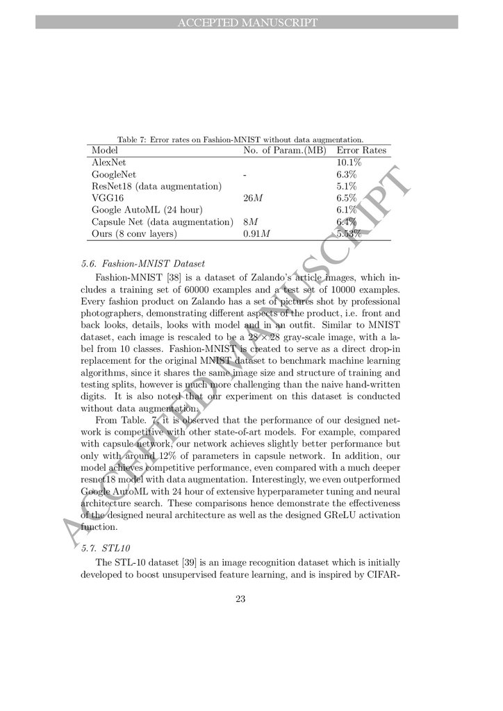
ACCEPTED MANUSCRIPT
Table 7: Error rates on Fashion-MNIST without data augmentation.
Error Rates
10.1%
6.3%
5.1%
6.5%
6.1%
6.4%
5.53%
CR
IP
T
Model
No. of Param.(MB)
AlexNet
GoogleNet
ResNet18 (data augmentation)
VGG16
26M
Google AutoML (24 hour)
Capsule Net (data augmentation) 8M
Ours (8 conv layers)
0.91M
AC
CE
PT
ED
M
AN
US
5.6. Fashion-MNIST Dataset
Fashion-MNIST [38] is a dataset of Zalando’s article images, which includes a training set of 60000 examples and a test set of 10000 examples.
Every fashion product on Zalando has a set of pictures shot by professional
photographers, demonstrating different aspects of the product, i.e. front and
back looks, details, looks with model and in an outfit. Similar to MNIST
dataset, each image is rescaled to be a 28 × 28 gray-scale image, with a label from 10 classes. Fashion-MNIST is created to serve as a direct drop-in
replacement for the original MNIST dataset to benchmark machine learning
algorithms, since it shares the same image size and structure of training and
testing splits, however is much more challenging than the naive hand-written
digits. It is also noted that our experiment on this dataset is conducted
without data augmentation.
From Table. 7, it is observed that the performance of our designed network is competitive with other state-of-art models. For example, compared
with capsule network, our network achieves slightly better performance but
only with around 12% of parameters in capsule network. In addition, our
model achieves competitive performance, even compared with a much deeper
resnet18 model with data augmentation. Interestingly, we even outperformed
Google AutoML with 24 hour of extensive hyperparameter tuning and neural
architecture search. These comparisons hence demonstrate the effectiveness
of the designed neural architecture as well as the designed GReLU activation
function.
5.7. STL10
The STL-10 dataset [39] is an image recognition dataset which is initially
developed to boost unsupervised feature learning, and is inspired by CIFAR23

26.

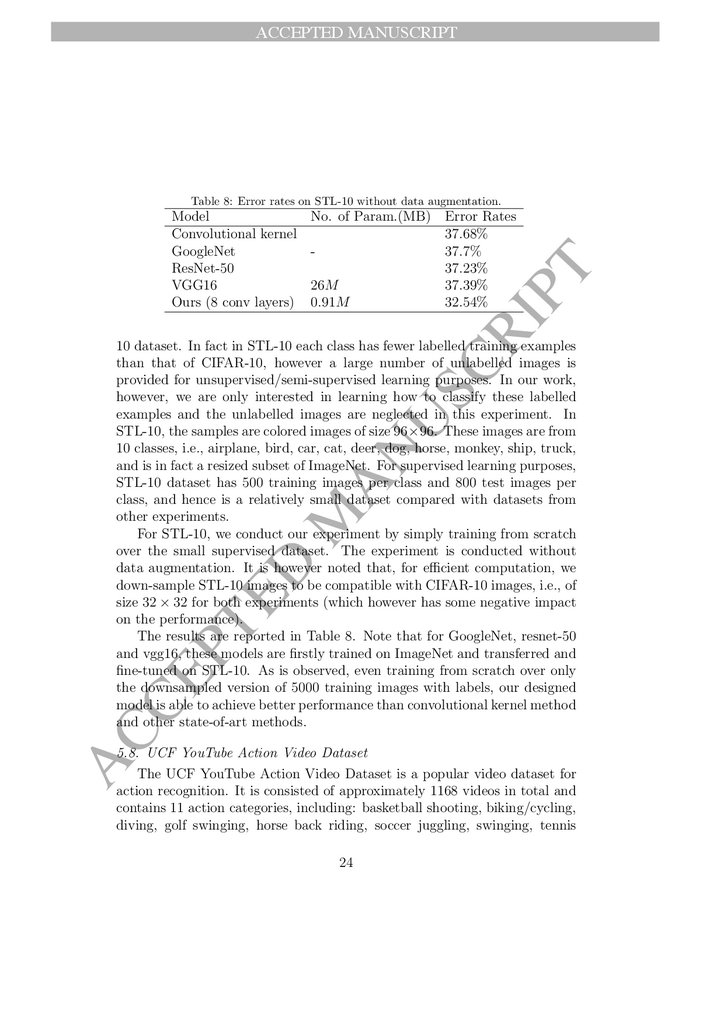
ACCEPTED MANUSCRIPT
Table 8: Error rates on STL-10 without data augmentation.
No. of Param.(MB)
26M
0.91M
Error Rates
37.68%
37.7%
37.23%
37.39%
32.54%
CR
IP
T
Model
Convolutional kernel
GoogleNet
ResNet-50
VGG16
Ours (8 conv layers)
AC
CE
PT
ED
M
AN
US
10 dataset. In fact in STL-10 each class has fewer labelled training examples
than that of CIFAR-10, however a large number of unlabelled images is
provided for unsupervised/semi-supervised learning purposes. In our work,
however, we are only interested in learning how to classify these labelled
examples and the unlabelled images are neglected in this experiment. In
STL-10, the samples are colored images of size 96×96. These images are from
10 classes, i.e., airplane, bird, car, cat, deer, dog, horse, monkey, ship, truck,
and is in fact a resized subset of ImageNet. For supervised learning purposes,
STL-10 dataset has 500 training images per class and 800 test images per
class, and hence is a relatively small dataset compared with datasets from
other experiments.
For STL-10, we conduct our experiment by simply training from scratch
over the small supervised dataset. The experiment is conducted without
data augmentation. It is however noted that, for efficient computation, we
down-sample STL-10 images to be compatible with CIFAR-10 images, i.e., of
size 32 × 32 for both experiments (which however has some negative impact
on the performance).
The results are reported in Table 8. Note that for GoogleNet, resnet-50
and vgg16, these models are firstly trained on ImageNet and transferred and
fine-tuned on STL-10. As is observed, even training from scratch over only
the downsampled version of 5000 training images with labels, our designed
model is able to achieve better performance than convolutional kernel method
and other state-of-art methods.
5.8. UCF YouTube Action Video Dataset
The UCF YouTube Action Video Dataset is a popular video dataset for
action recognition. It is consisted of approximately 1168 videos in total and
contains 11 action categories, including: basketball shooting, biking/cycling,
diving, golf swinging, horse back riding, soccer juggling, swinging, tennis
24

27.

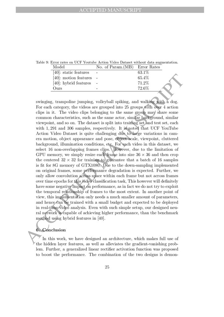
ACCEPTED MANUSCRIPT
Table 9: Error rates on UCF Youtube Action Video Dataset without data augmentation.
Error Rates
63.1%
65.4%
71.2%
72.6%
CR
IP
T
Model
No. of Param.(MB)
[40]: static features
[40]: motion features [40]: hybrid features Ours
-
AC
CE
PT
ED
M
AN
US
swinging, trampoline jumping, volleyball spiking, and walking with a dog.
For each category, the videos are grouped into 25 groups with over 4 action
clips in it. The video clips belonging to the same group may share some
common characteristics, such as the same actor, similar background, similar
viewpoint, and so on. The dataset is split into training set and test set, each
with 1, 291 and 306 samples, respectively. It is noted that UCF YouTube
Action Video Dataset is quite challenging due to large variations in camera motion, object appearance and pose, object scale, viewpoint, cluttered
background, illumination conditions, etc. For each video in this dataset, we
select 16 non-overlapping frames clips. However, due to the limitation of
GPU memory, we simply resize each frame into size 36 × 36 and then crop
the centered 32 × 32 for training to guarantee that a batch of 16 samples
is fit for 8G memory of GTX1080. Due to the down-sampling implemented
on original frames, some performance degradation is expected. Further, we
only allow convolution across space within each frame but not across frames
over time epochs for this video classification task, This however will definitely
have some negative impact on performance, as in fact we do not try to exploit
the temporal relationship of frames to the most extent. In another point of
view, this implementation only needs a much smaller amount of parameters,
and hence can be trained with a small budget and expected to be deployed
in real-time video analysis. Even with such simple setup, our designed neural network is capable of achieving higher performance, than the benchmark
method using hybrid features in [40].
6. Conclusion
In this work, we have designed an architecture, which makes full use of
the hidden layer features, as well as alleviates the gradient-vanishing problem. Further, a generalized linear rectifier activation function was proposed
to boost the performance. The combination of the two designs is demon25

28.

ACCEPTED MANUSCRIPT
PT
References
ED
M
AN
US
CR
IP
T
strated to achieve state of art performance in several object recognition and
video action recognition benchmark tasks, including MNIST, CIFAR-10/100,
SVHN, Fashion-MNIST, STL-10 and UCF YouTube Action video datasets,
with greatly reduced amount of parameters and even shallower structure.
Henceforth, our design can be employed in small-scale real-time application scenarios, as it requires less parameters and shallower network structure
whereas achieving matching/close performance with state-of-the-art models.
One can extend our work in several ways. Firstly, one can naturally incorporate our architecture and GReLU with other state-of-art architectures
such as resnet and densenet. These architectures are independent of ours as
they are more involved in the design of blocks of the deep neural networks,
while ours is on the flow of intermediate layers to final classification. In
this sense, one can merge these designs together to further improve performance by enjoying benefits of different works. Secondly, due to the fact that
different hidden layers provide feature information at different level, diving
deeper to utilize them instead of concatenation at the last layer would be of
great interest to investigate and expected to boost the performance as well.
Further, in this work, we do not tune the hyperparameters to optimize performance, one can fine tune these hyperparameters and observe their impact
on the designed network, e.g., optimization on the initialization of GReLU
parameters as well as learning rates. In addition, one can apply the designed
architecture to deeper neural networks and fine tune it in other interesting
computer vision tasks such as autonomous driving.
References
AC
CE
[1] O. Russakovsky, J. Deng, H. Su, J. Krause, S. Satheesh, S. Ma and
M. Bernstein. “ImageNet large scale visual recognition challenge”. International Journal of Computer Vision, vol. 115, no. 3, pp. 211-252,
2015.
[2] Y. LeCun and Y. Bengio and G. Hinton. “Deep learning”. Nature, vol.
521, no. 5, pp. 436-444, 2015.
[3] Y. Bengio, A. Courville and P. Vincent. “Representation learning: A
review and new perspectives”. IEEE Transactions on Pattern Analysis
and Machine Intelligence, vol. 35, no. 8, pp. 1798-1828, 2013.
26

29.

ACCEPTED MANUSCRIPT
[4] J. Schmidhuber. “Deep learning in neural networks: An overview”. Neural Networks, vol. 61, no. 1, pp. 85-117, 2015.
CR
IP
T
[5] Szegedy, C. et al. “Going deeper with convolutions”. In Proc. IEEE.
Computer Vision and Pattern Recognition (CVPR’15), 2015.
[6] K. He, X. Zhang, S. Ren, and J. Sun. “Deep residual learning for image recognition”. In Proc. IEEE Conf. Computer Vision and Pattern
Recognition (CVPR’16), pp. 770-778, 2016.
AN
US
[7] R. K. Srivastava, K. Greff, and J. Schmidhuber. “Training very deep
networks”. In Advances in Neural Information Processing Systems
(NIPS’15), pp. 2377-2385, 2015.
[8] P. Baldi and P. Sadowski. “The dropout learning algorithm”. Artificial
Intelligence, vol. 210, no. 5, pp. 78-122, 2014.
M
[9] Srivastava, N., Hinton, G., Krizhevsky, A., Sutskever, I. & Salakhutdinov, R. “Dropout: a simple way to prevent neural networks from
overfitting”. Journal of Machine Learning Research. vol. 15, no. 1, pp.
1929-1958 (2014).
ED
[10] S. Ioffe, & C. Szegedy, C. “Batch normalization: Accelerating deep network training by reducing internal covariate shift”. In Int. Conf. Machine Learning (ICML’15), 2015.
PT
[11] M. Gong, J. Liu, H. Li, Q. Cai, and L. Su, “A multiobjective sparse
feature learning model for deep neural networks,” IEEE Transaction on
Neural Networks and Learning System, vol. 26, no. 12, pp. 3263-3277,
Dec. 2015.
CE
[12] X. Glorot, A. Bordes & Y. Bengio. “Deep sparse rectifier neural networks”. In Proc. 14th Int. Conf. Artificial Intelligence and Statistics
(AISTATS’11), pp. 315-323 (2011).
AC
[13] A. L. Maas, A. Y. Hannun and A. Y. Ng. “Rectifier nonlinearities improve neural network acoustic models”. In Proc. Int. Conf. Machine
Learing (ICML’13), vol. 30, 2013.
[14] K. He, X. Zhang, S. Ren and J. Sun. “Delving Deep into Rectifiers:
Surpassing Human-Level Performance on Image Net Classification”. In
Proc. IEEE. Conf. Conference Vision (ICML’15), pp. 1026-1034, 2015.
27

30.

ACCEPTED MANUSCRIPT
[15] X. Jin, C. Xu, J. Feng, Y. Wei, J. Xiong and S. Yan. “Deep learning
with S-shaped rectified linear activation units”. In Thirtieth AAAI Conf.
Artificial Intelligence (AAAI’16). Feb 2016.
CR
IP
T
[16] D. Clevert, T. Unterthiner and S. Hochreiter. “Fast and Accurate Deep
Network Learning by Exponential Linear Units (ELUs)”, In Int. Conf.
Learning Representations (ICLR’16), 2016.
[17] I. J. Goodfellow, D. Warde-Farley, M. Mirza, A. Courville and Y. Bengio, Y. “Maxout networks”. In Proc. 30th Int. Conf. Machine Learning
(ICML’13). 2013.
AN
US
[18] K. Simonyan, & A. Zisserman, “Very deep convolutional networks for
large-scale image recognition”. In Proc. Int. Conf. Learning Representations (ICLR’14) ,2014.
[19] G. Huang, Y. Sun, Z. Liu, D. Sedra, and K. Q. Weinberger. “Deep
networks with stochastic depth”. In European Conf. Computer Vison
(ECCV’16), 2016.
M
[20] G. Larsson, M. Maire and G. Shakhnarovich. “Fractalnet: Ultra-deep
neural networks without residuals”. In Int. Conf. Learning Representation (ICLR’17), 2017.
ED
[21] S. Zagoruyko and N. Komodakis. “Wide residual networks”. In Proc.
the British Machine Vision Conference (BMVC’16), 2016.
PT
[22] G.E. Hinton, S. Sabour and N. Frosst, 2018. “Matrix capsules with EM
routing”, Int. Conf. Learning Representation (ICLR’18), 2018.
CE
[23] B. Hariharan, P. Arbelaez, R. Girshick and J. Malik. “Hypercolumns
for object segmentation and fine-grained localization”. In Proc. IEEE
Conf. Computer Vision and Pattern Recognition (CVPR’15), pp. 447456, 2015.
AC
[24] X. Bai, B. Shi, C. Zhang, X. Cai and L. Qi. “Text/non-text image classification in the wild with convolutional neural networks”. Pattern Recognition, vol. 66, no. 6, pp. 437-446, Jun. 2017.
[25] P. Tang, X. Wang, B. Shi, X. Bai, W. Liu and Z. Tu. “Deep FisherNet
for image classification”. IEEE Transactions on Neural Networks and
Learning Systems. early access, pp. 1-7, 2018.
28

31.

ACCEPTED MANUSCRIPT
[26] P. Tang, X. Wang, Z. Huang, X. Bai and W. Liu. “Deep patch learning for weakly supervised object classification and discovery”. Pattern
Recognition, vol. 71, no. 11, pp. 446-459, Nov, 2017.
CR
IP
T
[27] C. Hong, J. Yu, J. Wan, D. Tao and M. Wang. “Multimodal deep autoencoder for human pose recovery”. IEEE Transactions on Image Processing. vol. 24, no. 12, pp. 5659-5670, 2015.
[28] X. Wang, Y. Yan, P. Tang, X. Bai and W. Liu. “Revisiting multiple instance neural networks”. Pattern Recognition. vol. 74, no. 2, pp. 15-24,
2018.
AN
US
[29] J. Du and Y. Xu. “Hierarchical deep neural network for multivariate
regression”. Pattern Recognition. vol. 63, no. 3, pp. 149-157, 2017.
[30] J. Yu, B. Zhang, Z. Kuang, D. Lin and J. Fan. “iPrivacy: image privacy
protection by identifying sensitive objects via deep multi-task learning”.
IEEE Transactions on Information Forensics and Security. vol. 12, no.
5, pp. 1005-1016, 2017.
ED
M
[31] J. Yu, X. Yang, F. Gao and D. Tao. “Deep multimodal distance metric
learning using click constraints for image ranking”. IEEE Transactions
on Cybernetics. vol. 47, no. 12, pp. 4014-4024, 2017.
[32] M. Lin, Q. Chen and S. Yan. “Network in network”. In Proc. Int. Conf.
Learning Representation (ICLR’14), 2014.
CE
PT
[33] C.-Y. Lee, S. Xie, P. Gallagher, Z. Zhang and Z. Tu. “Deeply supervised nets”. In 18th Int. Conf. Artificial Intelligence and Statistics (AISTATS’15), 2015.
AC
[34] G. Huang, Z. Liu, K. Q. Weinberger and L. van der Maaten. “Densely
connected convolutional networks”. In Proc. IEEE Conf. Computer Vision and Pattern Recognition (CVPR’17), 2017.
[35] Y. LeCun, L. Bottou, Y. Bengio, and P. Haffner. “Gradient-based learning applied to document recognition.” Proceedings of the IEEE, vol. 86,
no. 11, pp. 2278-2324, Nov 1998.
[36] A. Krizhevsky and G. Hinton. “Learning multiple layers of features from
tiny images”, 2009.
29

32.

ACCEPTED MANUSCRIPT
[37] Y. Netzer, T. Wang, A. Coates, A. Bissacco, B. Wu, A. Y. Ng. “Reading
digits in natural images with unsupervised feature learning”, In NIPS
Workshop on Deep Learning and Unsupervised Feature Learning, 2011.
CR
IP
T
[38] H. Xiao, K. Rasul and R. Vollgraf, Fashion-mnist: a novel image dataset
for benchmarking machine learning algorithms. 2017.
[39] A. Coates, H. Lee, Andrew Y. Ng, An analysis of single layer networks
in unsupervised feature learning, In Int. Conf. Artificial Intelligence and
Statistics (AISTATS’11), 2011.
AC
CE
PT
ED
M
AN
US
[40] J. Liu, J. Luo and M. Shah, “Recognizing realistic actions from videos
’in the Wild’”, In IEEE Int. Conf. Computer Vision and Pattern Recognition (CVPR’09), 2009.
30

33.

ACCEPTED MANUSCRIPT
Dr. Zhi Chen received his B.S. degree from University of Electronic Science and Technology
of China in 2006, and the Ph.D. degree from Tsinghua University in 2011, all in Electrical
and Computer Engineering. Since January 2014, He has worked as a postdoctoral research
fellow with University of Waterloo's ECE Department. He has been a research associate in
the same group since Jan. 2016. His research interests span many areas including
communication and networking, internet of things, social networks, computer vision, deep
learning, and AI application development and deployment.
AC
CE
PT
ED
M
AN
US
CR
IP
T
Dr. Pin-Han Ho received his Ph.D. degree from Queen’s University at 2002. He is now a full
professor in the department of Electrical and Computer Engineering, University of Waterloo,
Canada. Professor Pin-Han Ho is the author/co-author of more than 350 refereed technical
papers, several book chapters, and the co-author of two books. His current research
interests cover a wide range of topics in broadband areas including social networks,
machine learning, internet of things, computer vision, smart city, as well as other emerging
areas in AI. He is the recipient of Distinguished Research Excellent Award in the ECE
department of University of Waterloo, Early Researcher Award (Premier Research
Excellence Award) in 2005, and many Best Paper Awards including SPECTS'02, ICC'05,
ICC'07, and the Outstanding Paper Award in HPSR’02.
1