2.04M

chap1_sec2

2.

FUNCTIONS AND MODELS
1.2
MATHEMATICAL MODELS:
A CATALOG OF
ESSENTIAL FUNCTIONS
In this section, we will learn about:
The purpose of mathematical models.

MATHEMATICAL MODELS
A mathematical model is a mathematical
description—often by means of a function
or an equation—of a real-world phenomenon
such as:
Size of a population
Demand for a product
Speed of a falling object
Life expectancy of a person at birth
Cost of emission reductions

4.

PURPOSE
The purpose of the model is to
understand the phenomenon and,
perhaps, to make predictions about
future behavior.

5.

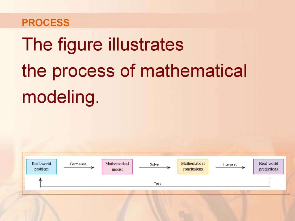
PROCESS
The figure illustrates
the process of mathematical
modeling.

6.

STAGE 1
Given a real-world problem, our first
task is to formulate a mathematical
model.
We do this by identifying and naming the
independent and dependent variables and
making assumptions that simplify the phenomenon
enough to make it mathematically tractable.

7.

STAGE 1
We use our knowledge of the physical
situation and our mathematical skills to
obtain equations that relate the variables.
In situations where there is no physical law to
guide us, we may need to collect data—from a
library, the Internet, or by conducting our own
experiments—and examine the data in the form
of a table in order to discern patterns.

8.

STAGE 1
From this numerical representation
of a function, we may wish to obtain
a graphical representation by plotting
the data.
In some cases, the graph might even suggest
a suitable algebraic formula.

9.

STAGE 2
The second stage is to apply the mathematics
that we know—such as the calculus that
will be developed throughout this book—to
the model that we have formulated in order to
derive mathematical conclusions.

10.

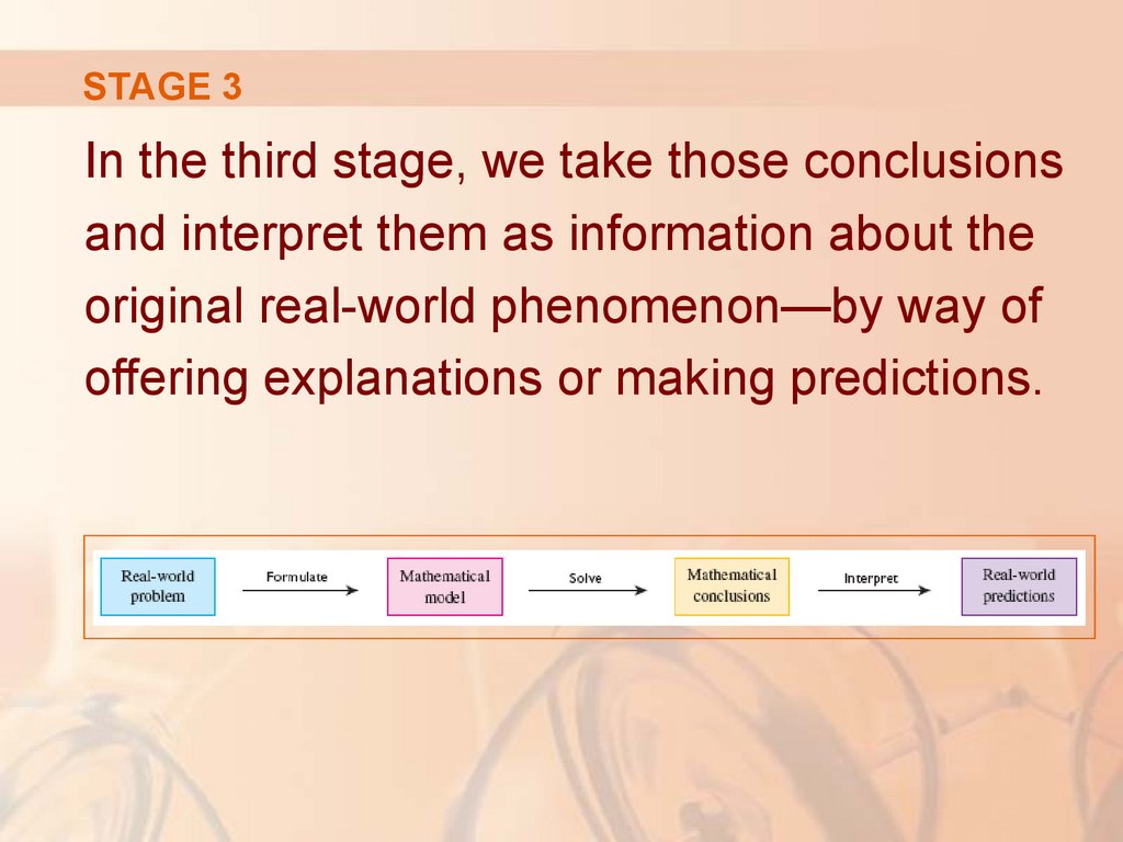
STAGE 3
In the third stage, we take those conclusions
and interpret them as information about the
original real-world phenomenon—by way of
offering explanations or making predictions.

11.

STAGE 4
The final step is to test our predictions
by checking against new real data.
If the predictions don’t compare well with reality,
we need to refine our model or to formulate
a new model and start the cycle again.

12.

MATHEMATICAL MODELS
A mathematical model is never a
completely accurate representation of a
physical situation—it is an idealization.
A good model simplifies reality enough to permit
mathematical calculations, but is accurate enough
to provide valuable conclusions.
It is important to realize the limitations of the model.
In the end, Mother Nature has the final say.

13.

MATHEMATICAL MODELS
There are many different types of
functions that can be used to model
relationships observed in the real world.
In what follows, we discuss the behavior and
graphs of these functions and give examples
of situations appropriately modeled by such functions.

14.

LINEAR MODELS
When we say that y is a linear
function of x, we mean that the graph
of the function is a line.
So, we can use the slope-intercept form of
the equation of a line to write a formula for
the function as
y = f ( x) = mx + b
where m is the slope of the line and b is
the y-intercept.

15.

LINEAR MODELS
A characteristic feature of
linear functions is that they grow
at a constant rate.

16.

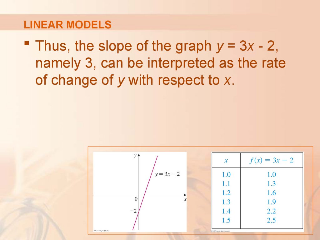
LINEAR MODELS
For instance, the figure shows a graph
of the linear function f(x) = 3x - 2 and
a table of sample values.
Notice that, whenever x increases by 0.1,
the value of f(x) increases by 0.3.
So, f (x) increases three times as fast as x.

17.

LINEAR MODELS
Thus, the slope of the graph y = 3x - 2,
namely 3, can be interpreted as the rate
of change of y with respect to x.

18.

LINEAR MODELS
Example 1
As dry air moves upward, it expands
and cools.
If the ground temperature is 20°C and the
temperature at a height of 1 km is 10°C,
express the temperature T (in °C) as a function
of the height h (in kilometers), assuming that
a linear model is appropriate.
Draw the graph of the function in part (a).
What does the slope represent?
What is the temperature at a height of 2.5 km?

19.

LINEAR MODELS
Example 1 a
As we are assuming that T is a linear
function of h, we can write T = mh + b.
We are given that T = 20 when h = 0,
so 20 = m . 0 + b = b.
In other words, the y-intercept is b = 20.
We are also given that T = 10 when h = 1,
so 10 = m . 1 + 20
Thus, the slope of the line is m = 10 – 20 = -10.
The required linear function is T = -10h + 20.

20.

LINEAR MODELS
Example 1 b
The slope is m = -10°C/km.
This represents the rate of change of
temperature with respect to height.

21.

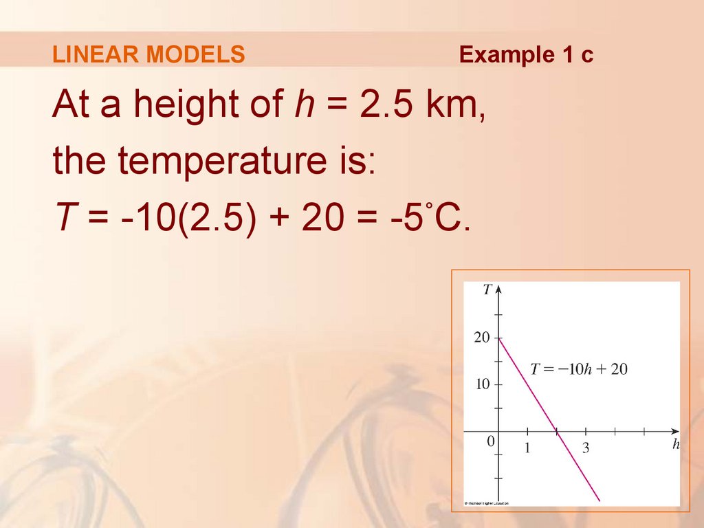
LINEAR MODELS
Example 1 c
At a height of h = 2.5 km,
the temperature is:
T = -10(2.5) + 20 = -5°C.

22.

EMPIRICAL MODEL
If there is no physical law or principle to
help us formulate a model, we construct
an empirical model.
This is based entirely on collected data.
We seek a curve that ‘fits’ the data in the sense
that it captures the basic trend of the data points.

23.

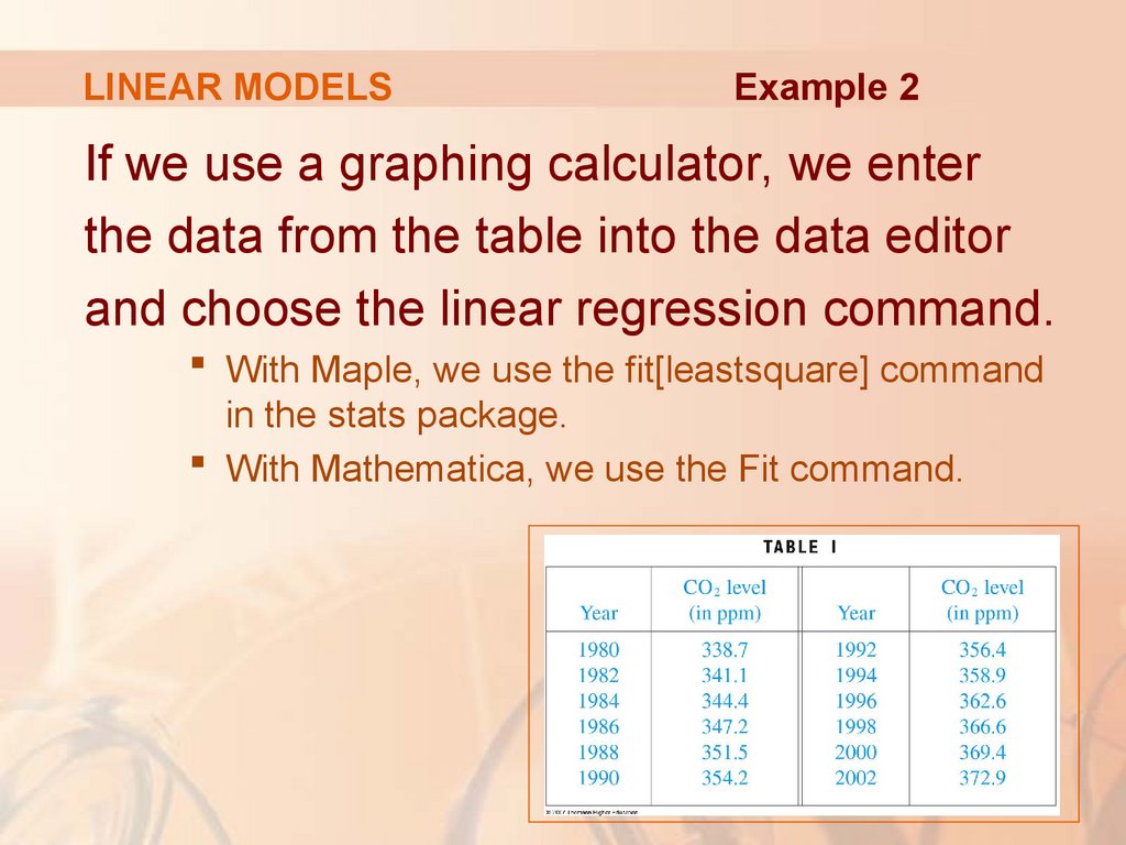
LINEAR MODELS
Example 2
The table lists the average carbon dioxide
(CO2) level in the atmosphere, measured in
parts per million at Mauna Loa Observatory
from 1980 to 2002.
Use the data to find a model for the CO2 level.

24.

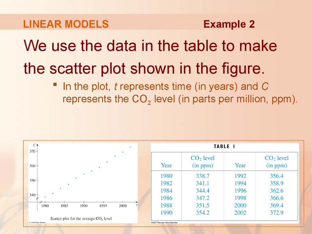
LINEAR MODELS
Example 2
We use the data in the table to make
the scatter plot shown in the figure.
In the plot, t represents time (in years) and C
represents the CO2 level (in parts per million, ppm).

25.

LINEAR MODELS
Example 2
Notice that the data points appear
to lie close to a straight line.
So, in this case, it’s natural to choose
a linear model.

26.

LINEAR MODELS
Example 2
However, there are many possible
lines that approximate these data points.
So, which one should we use?

27.

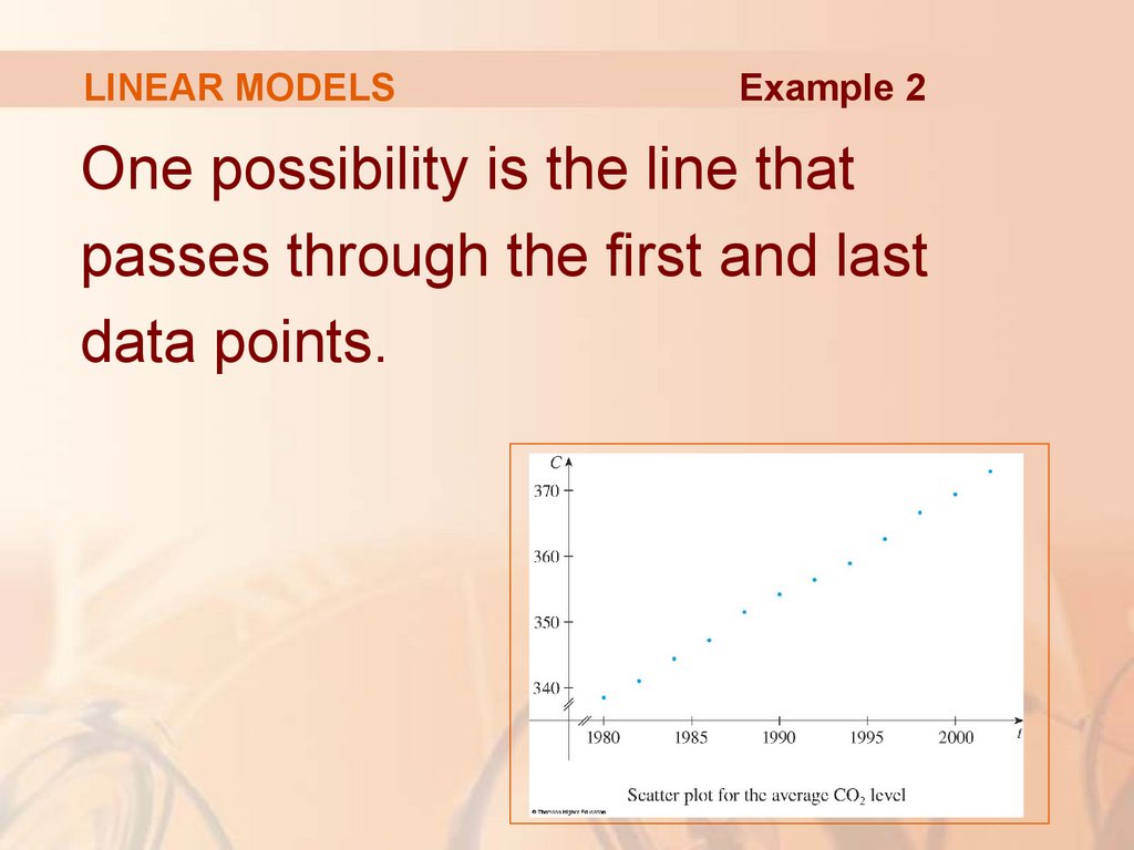
LINEAR MODELS
Example 2
One possibility is the line that
passes through the first and last
data points.

28.

LINEAR MODELS
The slope of this line is:
372.9 −338.7 34.2
=
≈1.5545
2002 −1980
22
Example 2

29.

LINEAR MODELS
E.g. 2—Equation 1
The equation of the line is:
C - 338.7 = 1.5545(t -1980)
or C = 1.5545t - 2739.21

30.

LINEAR MODELS
Example 2
This equation gives one possible linear
model for the CO2 level.
It is graphed in the figure.

31.

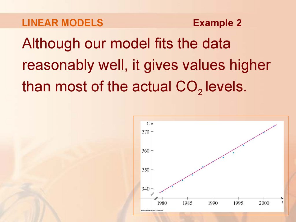
LINEAR MODELS
Example 2
Although our model fits the data
reasonably well, it gives values higher
than most of the actual CO2 levels.

32.

LINEAR MODELS
Example 2
A better linear model is obtained
by a procedure from statistics called
linear regression.

33.

LINEAR MODELS
Example 2
If we use a graphing calculator, we enter
the data from the table into the data editor
and choose the linear regression command.
With Maple, we use the fit[leastsquare] command
in the stats package.
With Mathematica, we use the Fit command.

34.

LINEAR MODELS
E. g. 2—Equation 2
The machine gives the slope and y-intercept
of the regression line as:
m = 1.55192
b = -2734.55
So, our least squares model for the level
CO2 is:
C = 1.55192t - 2734.55

35.

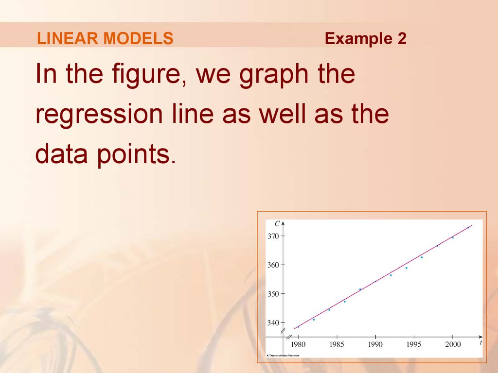
LINEAR MODELS
Example 2
In the figure, we graph the
regression line as well as the
data points.

36.

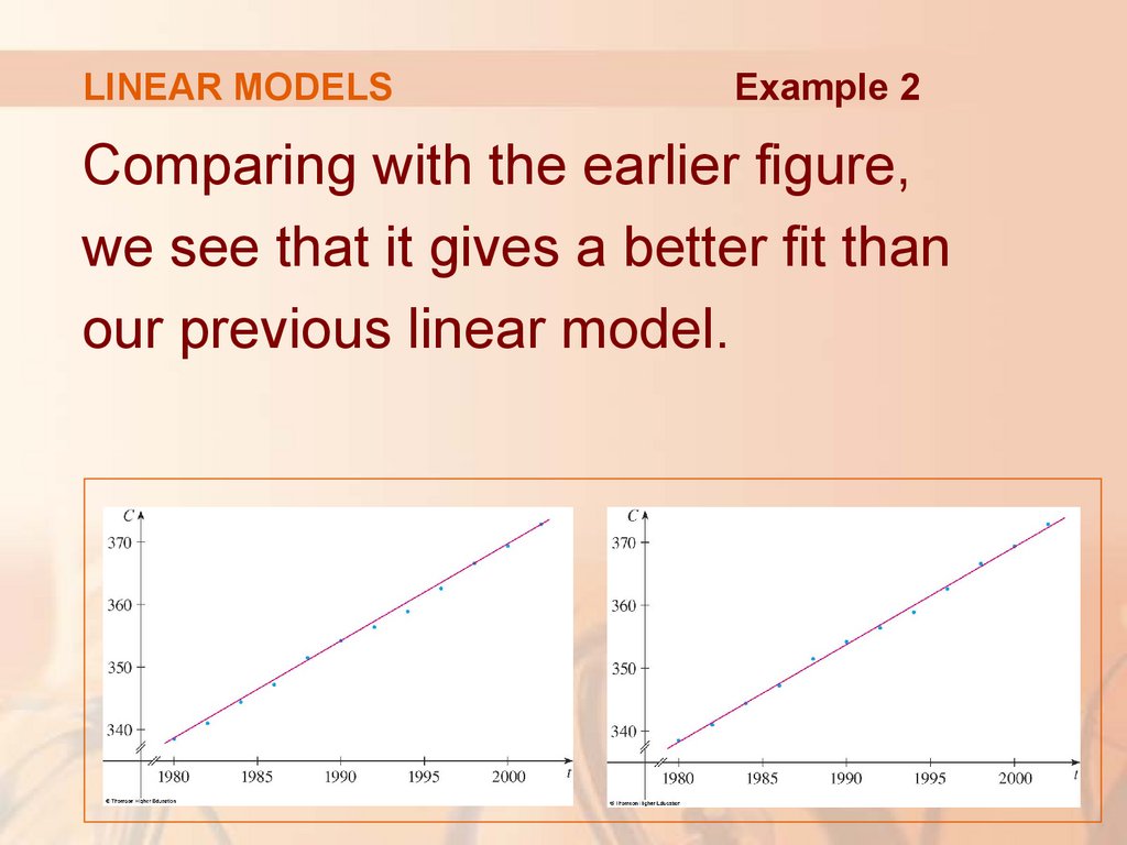
LINEAR MODELS
Example 2
Comparing with the earlier figure,
we see that it gives a better fit than
our previous linear model.

37.

LINEAR MODELS
Example 3
Use the linear model given by
Equation 2 to estimate the average
CO2 level for 1987 and to predict
the level for 2010.
According to this model, when will the CO2 level
exceed 400 parts per million?

38.

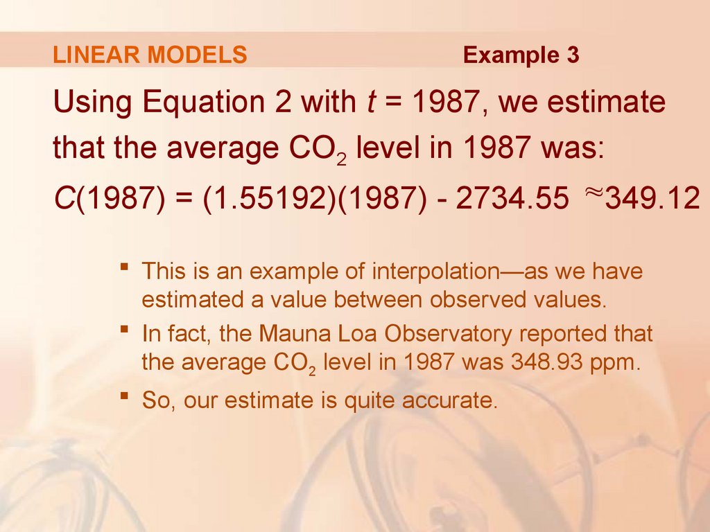
LINEAR MODELS
Example 3
Using Equation 2 with t = 1987, we estimate
that the average CO2 level in 1987 was:
C(1987) = (1.55192)(1987) - 2734.55 ≈349.12
This is an example of interpolation—as we have
estimated a value between observed values.
In fact, the Mauna Loa Observatory reported that
the average CO2 level in 1987 was 348.93 ppm.
So, our estimate is quite accurate.

39.

LINEAR MODELS
Example 3
With t = 2010, we get:
C(2010) = (1.55192)(2010) - 2734.55 ≈ 384.81
So, we predict that the average CO2 level in
2010 will be 384.8 ppm.
This is an example of extrapolation—as we have
predicted a value outside the region of observations.
Thus, we are far less certain about the accuracy
of our prediction.

40.

LINEAR MODELS
Example 3
Using Equation 2, we see that the CO2 level
exceeds 400 ppm when:
1.55192t −2734.55 > 400
Solving this inequality, we get:
3134.55
t>
≈2019.79
1.55192
Thus, we predict that the CO2 level
will exceed 400 ppm by 2019.
This prediction is somewhat risky—as it involves
a time quite remote from our observations.

41.

POLYNOMIALS
A function P is called a polynomial if
P(x) = anxn + an-1xn-1 + … + a2x2 + a1x + a0
where n is a nonnegative integer and
the numbers a0, a1, a2, …, an are constants
called the coefficients of the polynomial.

42.

POLYNOMIALS
The domain of any polynomial is ° = (−∞,∞).
If the leading coefficient an ≠0, then
the degree of the polynomial is n.
For example, the function
2 3
P ( x ) = 2 x −x + x + 2
5
6
4
is a polynomial of degree 6.

43.

DEGREE 1
A polynomial of degree 1 is of the form
P(x) = mx + b
So, it is a linear function.

44.

DEGREE 2
A polynomial of degree 2 is of the form
P(x) = ax2 + bx + c
It is called a quadratic function.

45.

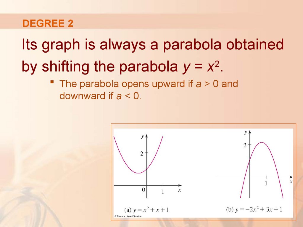
DEGREE 2
Its graph is always a parabola obtained
by shifting the parabola y = x2.
The parabola opens upward if a > 0 and
downward if a < 0.

46.

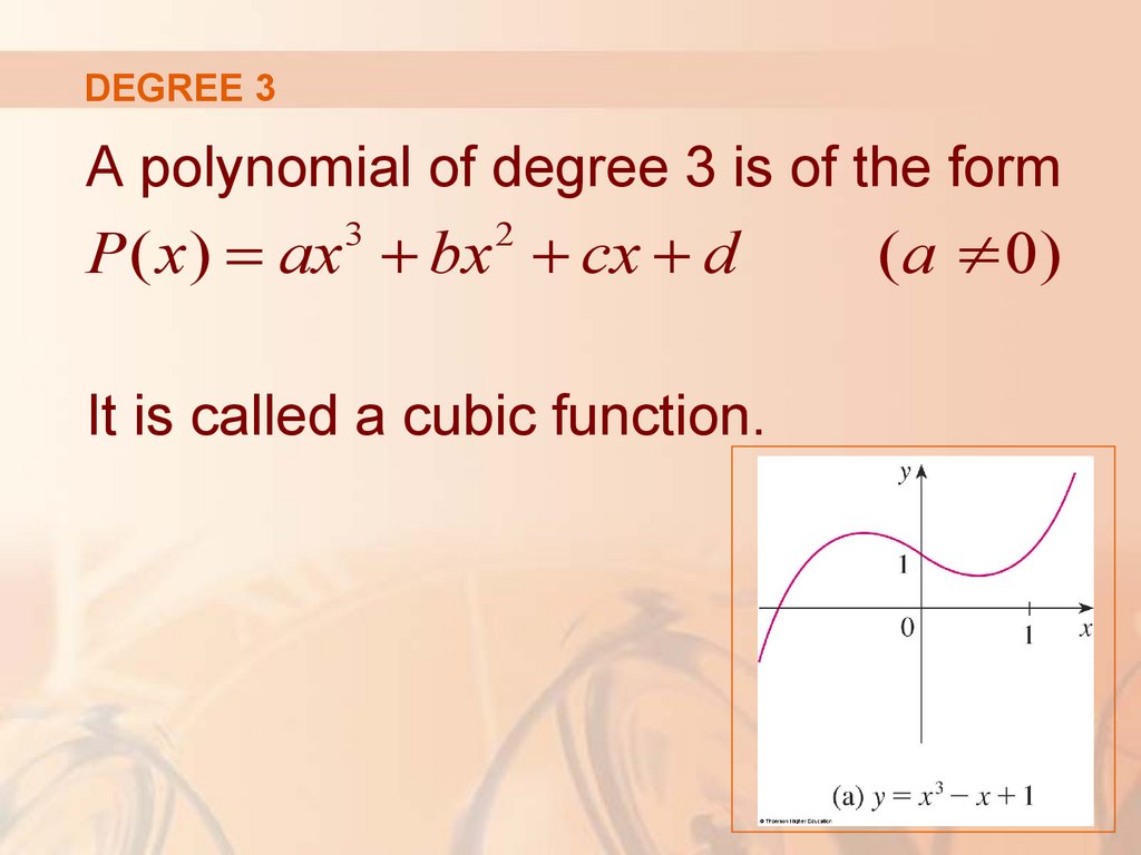
DEGREE 3
A polynomial of degree 3 is of the form
3
2
P ( x ) = ax + bx + cx + d
It is called a cubic function.
(a ≠0)

47.

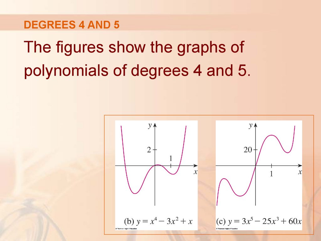
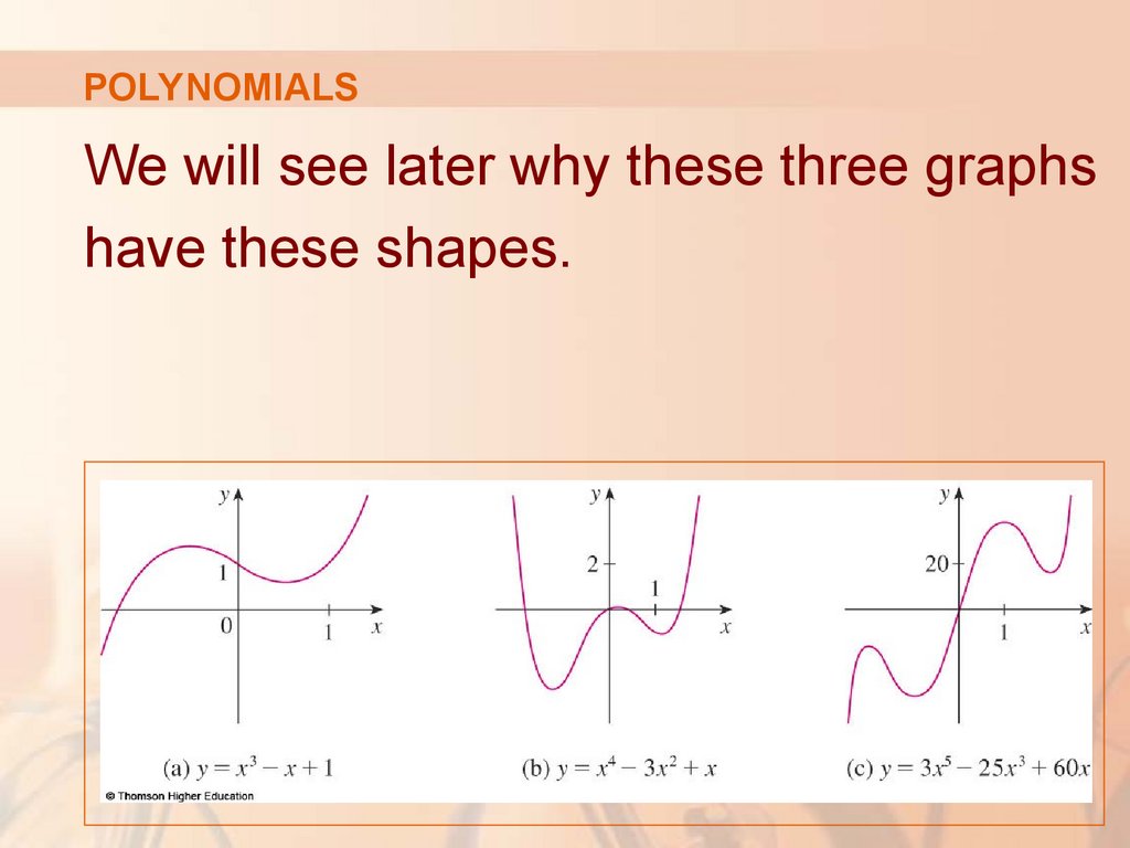
DEGREES 4 AND 5
The figures show the graphs of
polynomials of degrees 4 and 5.

48.

POLYNOMIALS
We will see later why these three graphs
have these shapes.

49.

POLYNOMIALS
Polynomials are commonly used to
model various quantities that occur
in the natural and social sciences.
For instance, in Section 3.7, we will explain
why economists often use a polynomial P(x)
to represent the cost of producing x units of
a commodity.
In the following example, we use a quadratic
function to model the fall of a ball.

50.

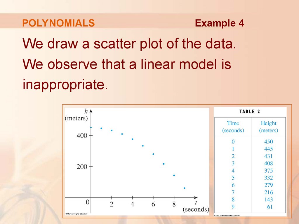
POLYNOMIALS
Example 4
A ball is dropped from the upper observation
deck of the CN Tower—450 m above the
ground—and its height h above the ground is
recorded at 1-second intervals.
Find a model to fit the data
and use the model to predict
the time at which the ball
hits the ground.

51.

POLYNOMIALS
Example 4
We draw a scatter plot of the data.
We observe that a linear model is
inappropriate.

52.

POLYNOMIALS
Example 4
However, it looks as if the data points
might lie on a parabola.
So, we try a quadratic model instead.

53.

POLYNOMIALS
E. g. 4—Equation 3
Using a graphing calculator or computer
algebra system (which uses the least squares
method), we obtain the following quadratic
model:
h = 449.36 + 0.96t - 4.90t2

54.

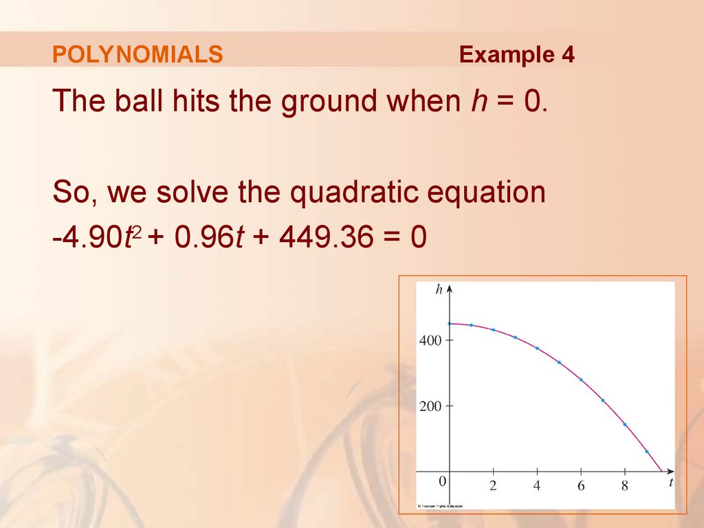
POLYNOMIALS
Example 4
We plot the graph of Equation 3 together
with the data points.
We see that the quadratic model gives
a very good fit.

55.

POLYNOMIALS
Example 4
The ball hits the ground when h = 0.
So, we solve the quadratic equation
-4.90t2 + 0.96t + 449.36 = 0

56.

POLYNOMIALS
Example 4
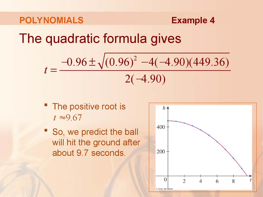
The quadratic formula gives
−0.96 ± (0.96) 2 −4(−4.90)(449.36)
t=
2(−4.90)
The positive root is
t ≈9.67
So, we predict the ball
will hit the ground after
about 9.7 seconds.

57.

POWER FUNCTIONS
A function of the form f(x) = xa,
where a is constant, is called a
power function.
We consider several cases.

58.

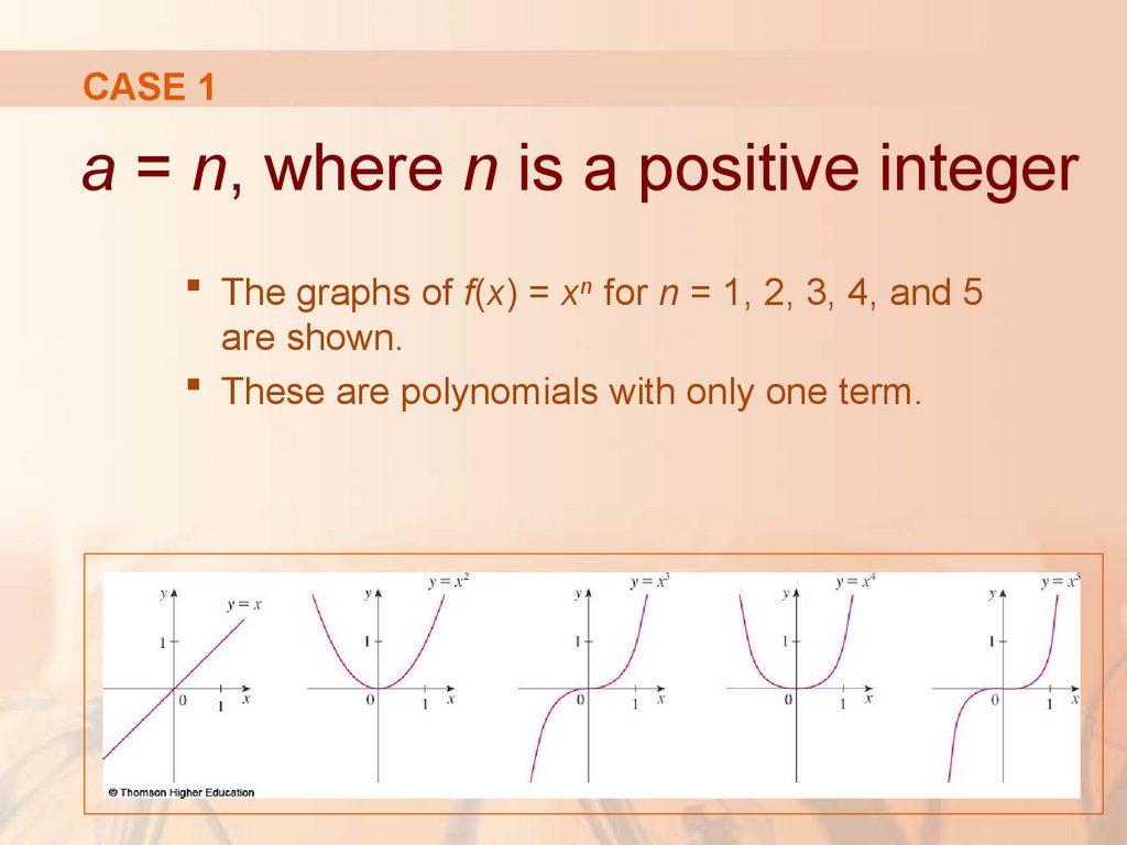
CASE 1
a = n, where n is a positive integer
The graphs of f(x) = xn for n = 1, 2, 3, 4, and 5
are shown.
These are polynomials with only one term.

59.

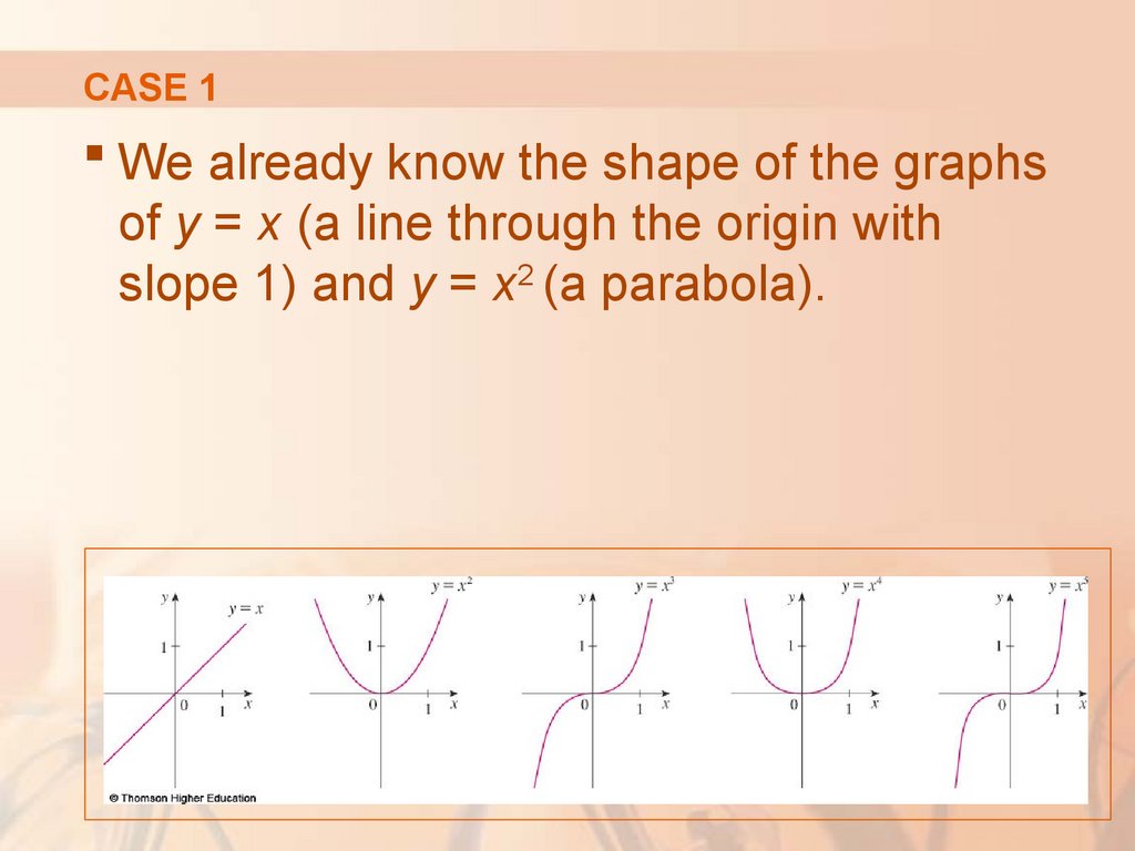
CASE 1
We already know the shape of the graphs
of y = x (a line through the origin with
slope 1) and y = x2 (a parabola).

60.

CASE 1
The general shape of the graph
of f(x) = xn depends on whether n
is even or odd.

61.

CASE 1
If n is even, then f(x) = xn is an even
function, and its graph is similar to
the parabola y = x2.

62.

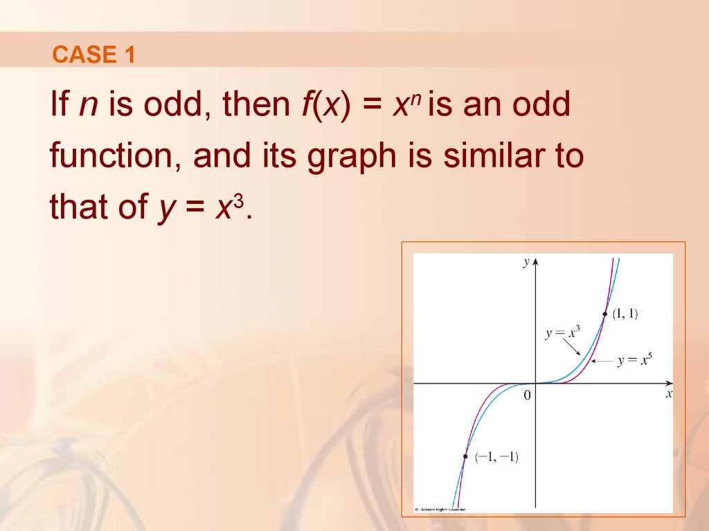
CASE 1
If n is odd, then f(x) = xn is an odd
function, and its graph is similar to
that of y = x3.

63.

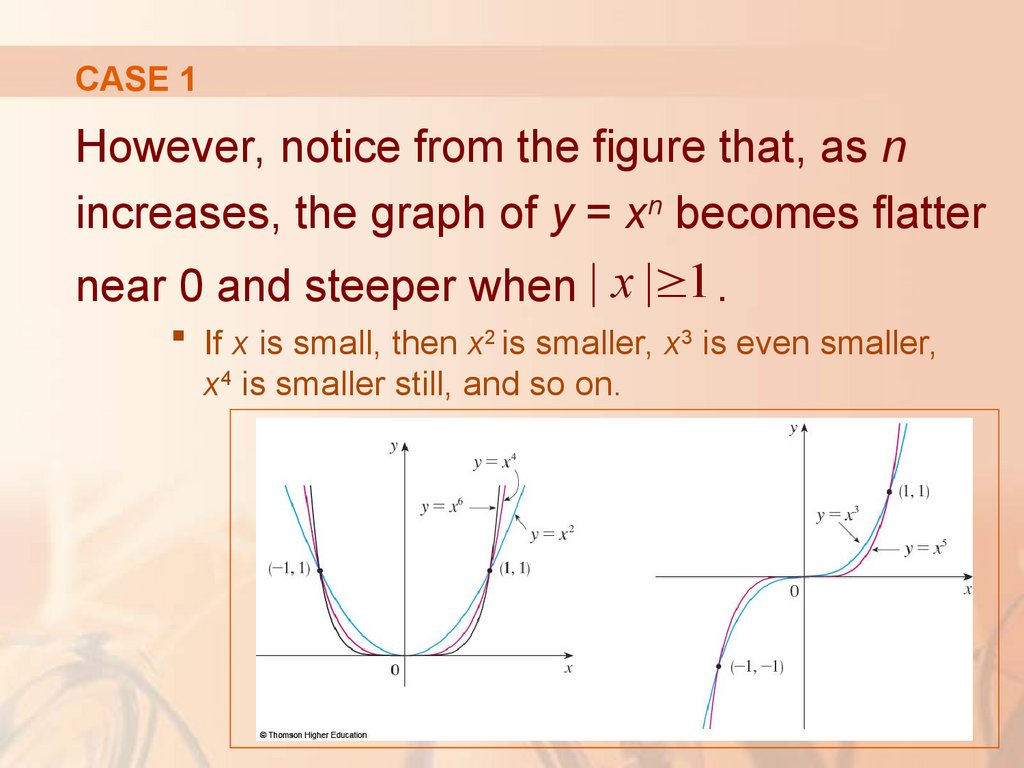
CASE 1
However, notice from the figure that, as n
increases, the graph of y = xn becomes flatter
near 0 and steeper when | x |≥1 .
If x is small, then x2 is smaller, x3 is even smaller,
x4 is smaller still, and so on.

64.

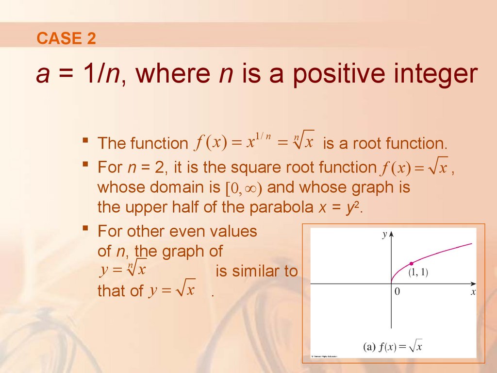
CASE 2
a = 1/n, where n is a positive integer
The function f ( x) = x1/ n = n x is a root function.
For n = 2, it is the square root function f ( x) = x ,
whose domain is [0, ∞) and whose graph is
the upper half of the parabola x = y2.
For other even values
of n, the graph of
y=nx
is similar to
that of y = x .

65.

CASE 2
For n = 3, we have the cube root function
f ( x) = 3 x whose domain is° (recall that
every
real number has a cube root) and whose
n
y
=
x
graph is shown. 3
= x
The graphy of
for n odd (n > 3) is similar
to that of
.

66.

CASE 3
a = -1
The graph of the reciprocal function f(x) = x-1 = 1/x
is shown.
Its graph has the equation y = 1/x, or xy = 1.
It is a hyperbola with
the coordinate axes as
its asymptotes.

67.

CASE 3
This function arises in physics and chemistry
in connection with Boyle’s Law, which states
that, when the temperature is constant, the
volume V of a gas is inversely proportional
to the pressure P.
C
V =
P
where C is a constant.

68.

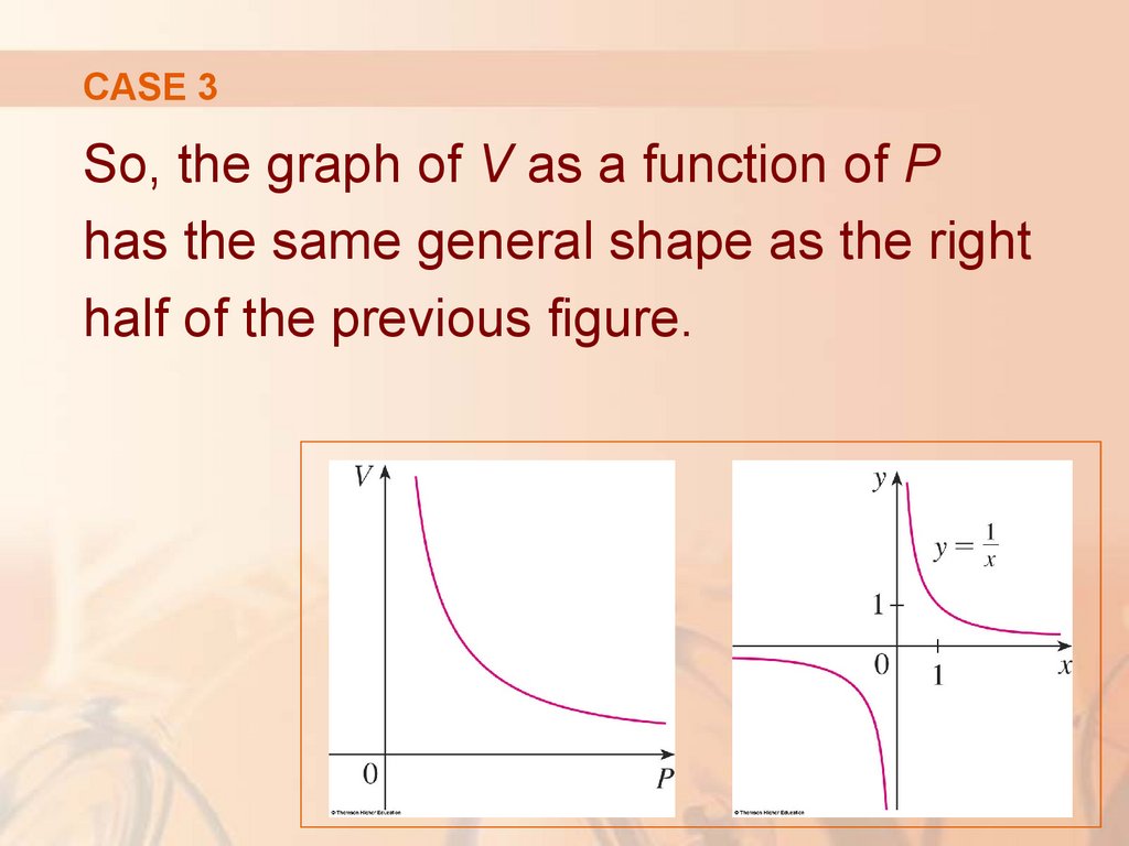
CASE 3
So, the graph of V as a function of P
has the same general shape as the right
half of the previous figure.

69.

RATIONAL FUNCTIONS
A rational function f is a ratio of two
P( x)
polynomials
f ( x) =
Q( x)
where P and Q are polynomials.
The domain consists of all values of x
such that Q( x) ≠0 .

70.

RATIONAL FUNCTIONS
A simple example of a rational function
is the function f(x) = 1/x, whose domain
is {x | x ≠ 0} .
This is the reciprocal function
graphed in the figure.

71.

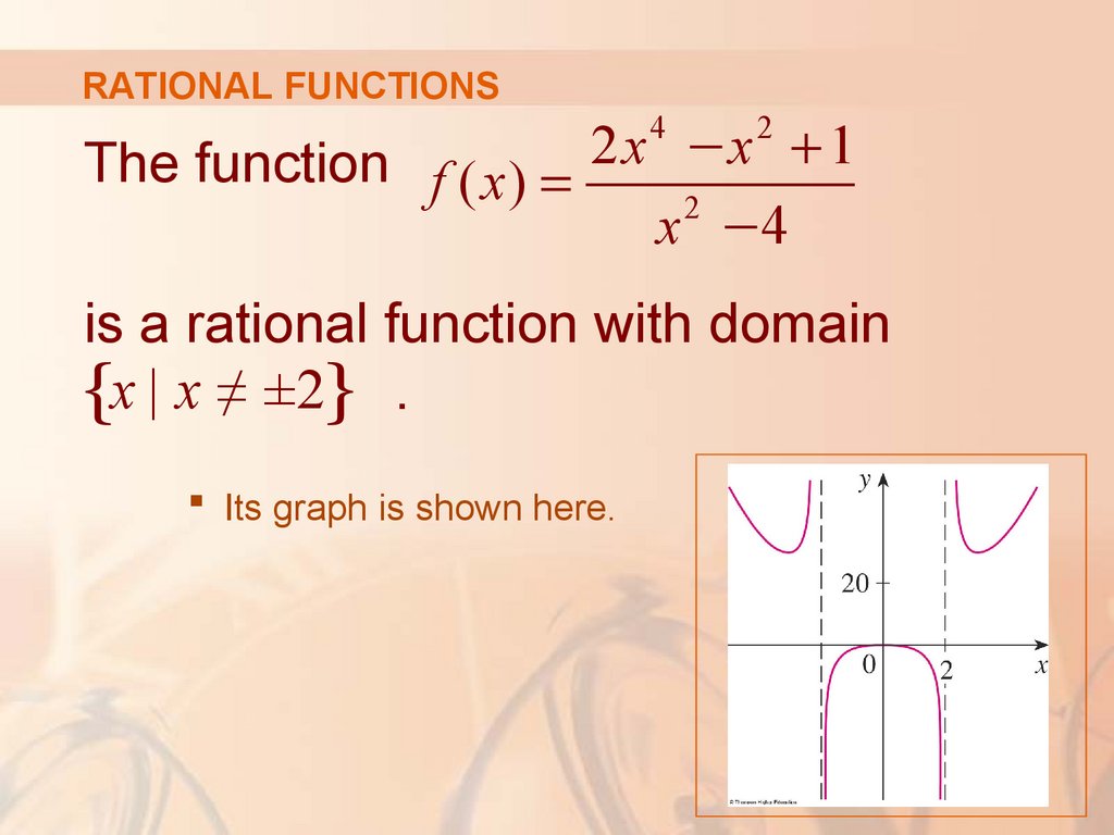
RATIONAL FUNCTIONS
4
2
The function f ( x) = 2 x −x + 1
2
x −4
is a rational function with domain
{x | x ≠ ±2} .
Its graph is shown here.

72.

ALGEBRAIC FUNCTIONS
A function f is called an algebraic function
if it can be constructed using algebraic
operations—such as addition, subtraction,
multiplication, division, and taking roots—
starting with polynomials.

73.

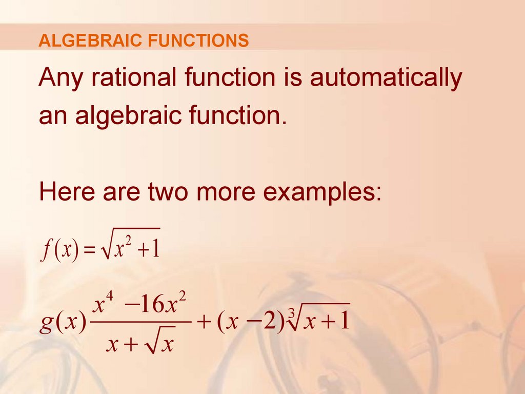
ALGEBRAIC FUNCTIONS
Any rational function is automatically
an algebraic function.
Here are two more examples:
2
f ( x) = x + 1
g ( x)
4
x −16 x
x+ x
2
3
+ ( x −2) x + 1

74.

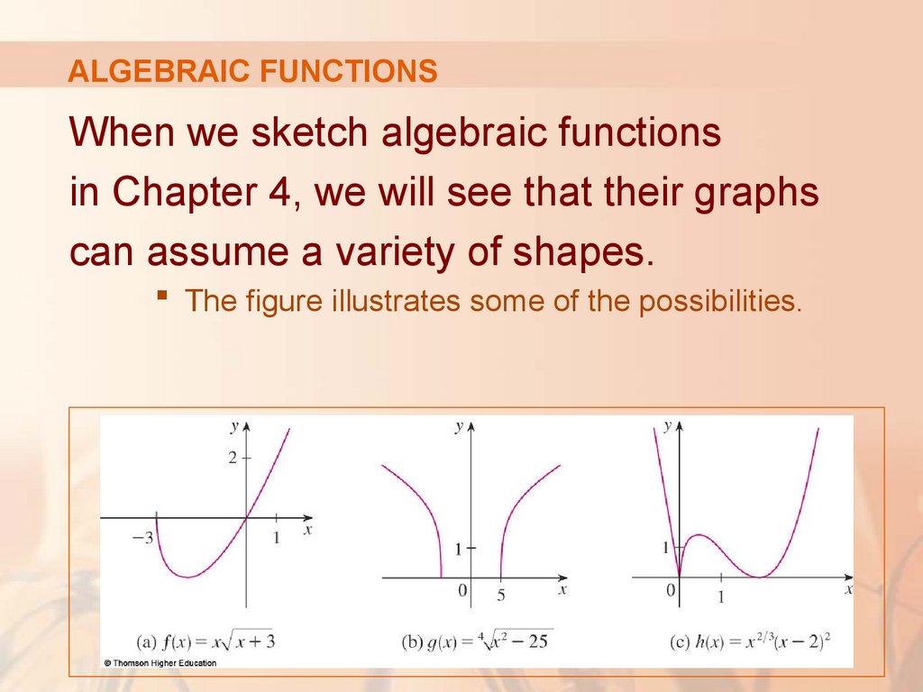
ALGEBRAIC FUNCTIONS
When we sketch algebraic functions
in Chapter 4, we will see that their graphs
can assume a variety of shapes.
The figure illustrates some of the possibilities.

75.

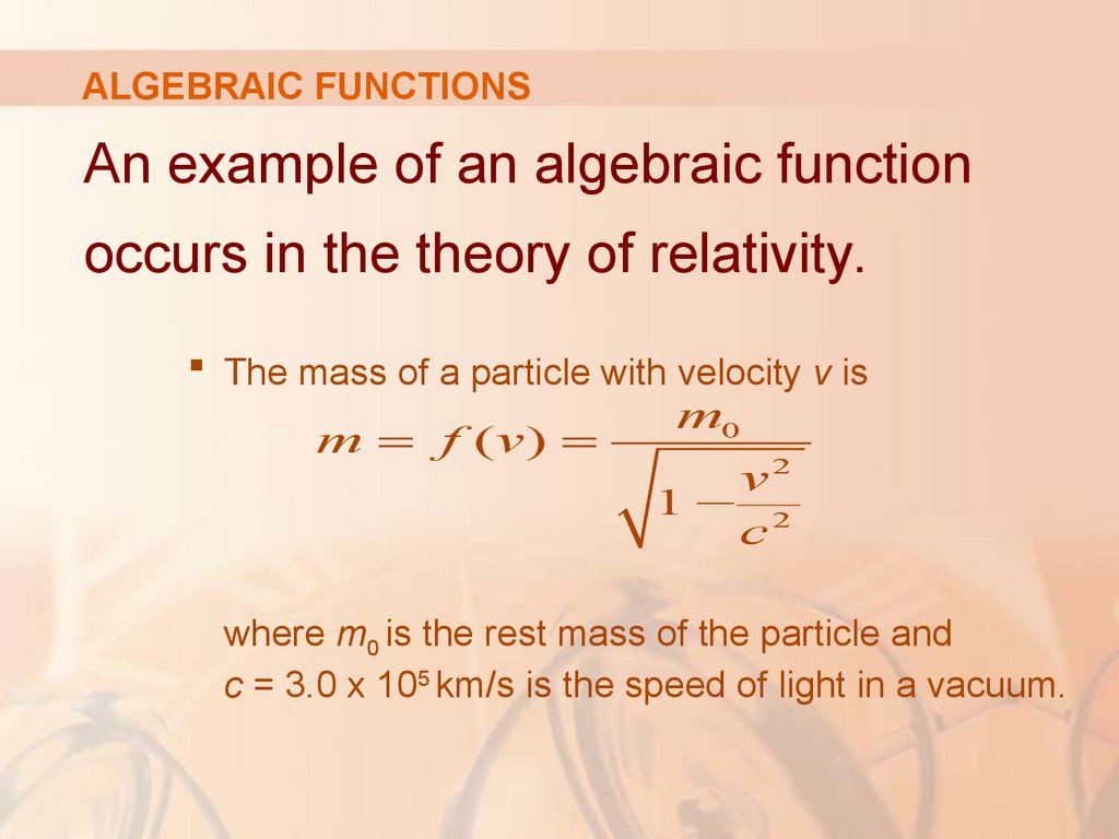
ALGEBRAIC FUNCTIONS
An example of an algebraic function
occurs in the theory of relativity.
The mass of a particle with velocity v is
m0
m = f (v ) =
v2
1− 2
c
where m0 is the rest mass of the particle and
c = 3.0 x 105 km/s is the speed of light in a vacuum.

76.

TRIGONOMETRIC FUNCTIONS
In calculus, the convention is that radian
measure is always used (except when
otherwise indicated).
For example, when we use the function f(x) = sin x,
it is understood that sin x means the sine of the
angle whose radian measure is x.

77.

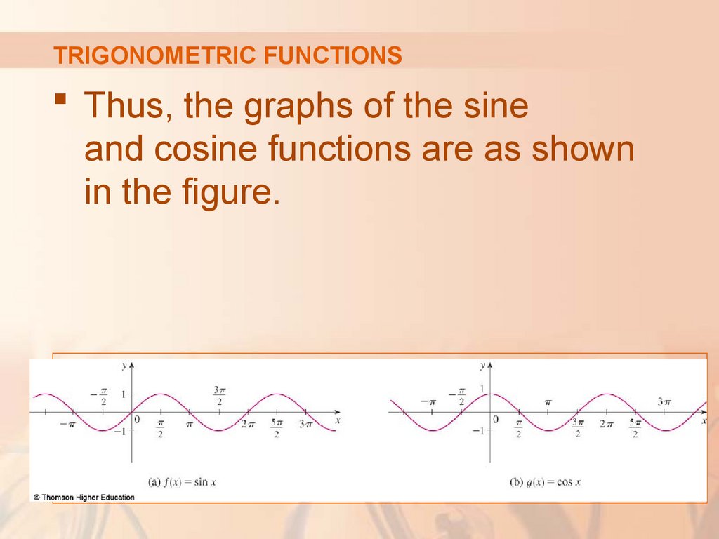
TRIGONOMETRIC FUNCTIONS
Thus, the graphs of the sine
and cosine functions are as shown
in the figure.

78.

TRIGONOMETRIC FUNCTIONS
Notice that, for both the sine and cosine
functions, the domain is (−∞, ∞) and the range
is the closed interval [-1, 1].
Thus, for all values of x, we have:
−1 ≤sin x ≤1
−1 ≤cos x ≤1
In terms of absolute values, it is: | sin x |≤1
| cos x |≤1

79.

TRIGONOMETRIC FUNCTIONS
Also, the zeros of the sine function
occur at the integer multiples of π .
That is, sin x = 0 when x = n π ,
n an integer.

80.

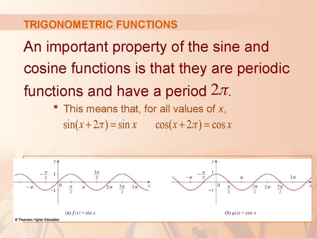
TRIGONOMETRIC FUNCTIONS
An important property of the sine and
cosine functions is that they are periodic
functions and have a period 2π.
This means that, for all values of x,
sin( x + 2π ) = sin x
cos( x + 2π ) = cos x

81.

TRIGONOMETRIC FUNCTIONS
The periodic nature of these functions
makes them suitable for modeling
repetitive phenomena such as tides,
vibrating springs, and sound waves.

82.

TRIGONOMETRIC FUNCTIONS
For instance, in Example 4 in Section 1.3,
we will see that a reasonable model for
the number of hours of daylight in Philadelphia
t days after January 1 is given by the function:
⎡ 2π
⎤
L(t ) = 12 + 2.8sin ⎢ (t −80) ⎥
⎣365
⎦

83.

TRIGONOMETRIC FUNCTIONS
The tangent function is related to
the sine and cosine functions by
sin x
the equation tan x =
cos x
Its graph is shown.

84.

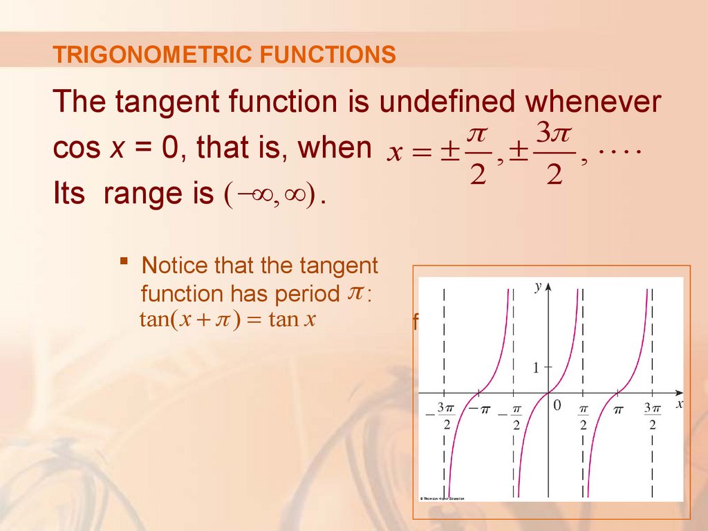
TRIGONOMETRIC FUNCTIONS
The tangent function is undefined whenever
π
3π
cos x = 0, that is, when x = ± , ±
, ⋅⋅⋅⋅
2
2
Its range is (−∞, ∞) .
Notice that the tangent
function has period π :
tan( x + π ) = tan x
for all x.

85.

TRIGONOMETRIC FUNCTIONS
The remaining three trigonometric
functions—cosecant, secant, and
cotangent—are the reciprocals of
the sine, cosine, and tangent functions.

86.

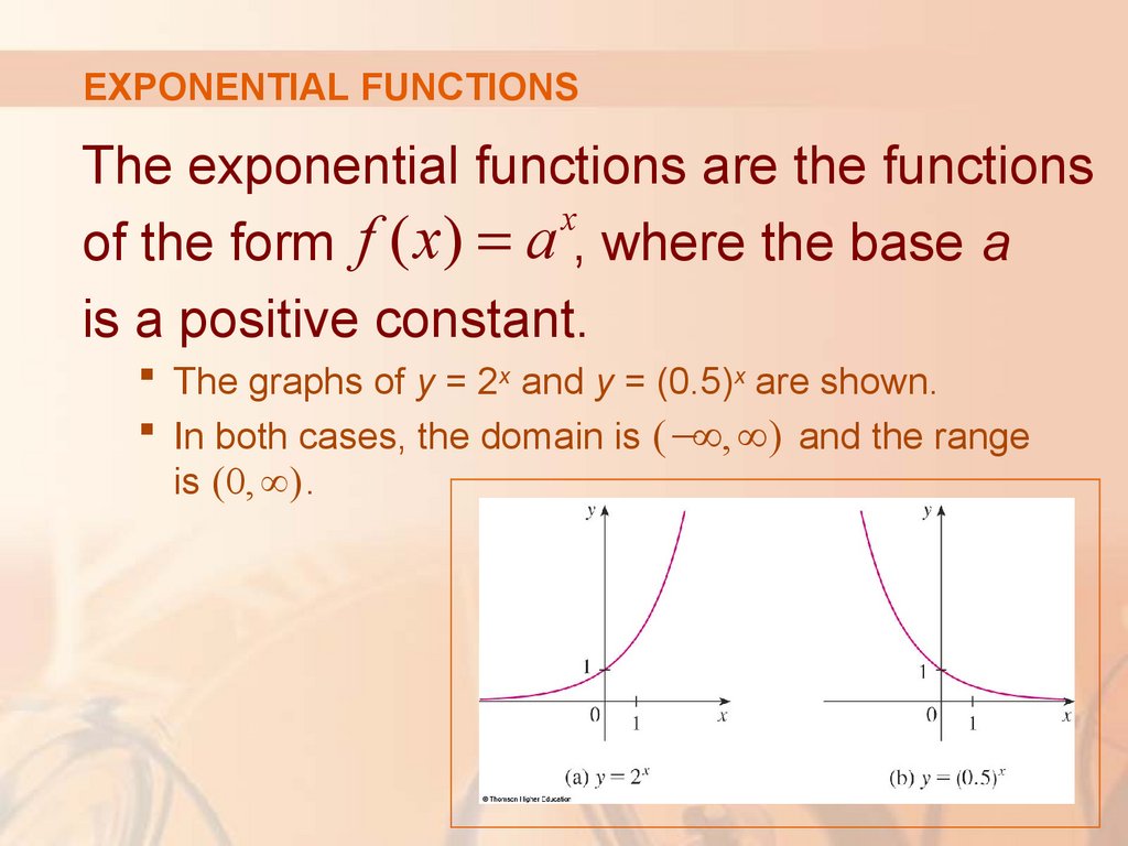
EXPONENTIAL FUNCTIONS
The exponential functions are the functions
x
of the form f ( x ) = a , where the base a
is a positive constant.
The graphs of y = 2x and y = (0.5)x are shown.
In both cases, the domain is (−∞, ∞) and the range
is (0, ∞) .

87.

EXPONENTIAL FUNCTIONS
We will study exponential functions
in detail in Section 1.5.
We will see that they are useful for modeling many
natural phenomena—such as population growth
(if a > 1) and radioactive decay (if a < 1).

88.

LOGARITHMIC FUNCTIONS
The logarithmic functions f ( x) = log a x,
where the base a is a positive constant,
are the inverse functions of the
exponential functions.
We will study them in Section 1.6.

89.

LOGARITHMIC FUNCTIONS
The figure shows the graphs of four
logarithmic functions with various bases.
In each case, the domain is (0, ∞) , the range is (−∞, ∞) ,
and the function increases slowly when x > 1.

90.

TRANSCENDENTAL FUNCTIONS
Transcendental functions are
those that are not algebraic.
The set of transcendental functions includes the
trigonometric, inverse trigonometric, exponential, and
logarithmic functions.
However, it also includes a vast number of other
functions that have never been named.
In Chapter 11, we will study transcendental functions
that are defined as sums of infinite series.