Functions and models. The fundamental objects that we deal with in calculus

1.

1
FUNCTIONS AND MODELS

2.

FUNCTIONS AND MODELS
The fundamental objects
that we deal with in calculus
are functions.

3.

FUNCTIONS AND MODELS
This chapter prepares the way
for calculus by discussing:
The basic ideas concerning functions
Their graphs
Ways of transforming and combining them

4.

FUNCTIONS AND MODELS
We stress that a function can be
represented in different ways:
By an equation
In a table
By a graph
In words

5.

FUNCTIONS AND MODELS
In this chapter, we:
Look at the main types of functions that occur
in calculus
Describe the process of using these functions as
mathematical models of real-world phenomena
Discuss the use of graphing calculators and
graphing software for computers

6.

FUNCTIONS AND MODELS
1.1
Four Ways to
Represent a Function
In this section, we will learn about:
The main types of functions that occur in calculus.

7.

FOUR WAYS TO REPRESENT A FUNCTION
Functions arise whenever
one quantity depends on
another.
Consider the following four situations.

8.

EXAMPLE A
The area A of a circle depends
on the radius r of the circle.
The rule that connects r and A is given by the
2
A
r
equation
.
With each positive number r, there is associated
one value of A, and we say that A is a function of r.

9.

EXAMPLE B
The human population of the world
P depends on the time t.
The table gives estimates of the
world population P(t) at time t,
for certain years.
For instance,
P(1950) 2,560, 000, 000
However, for each value of the
time t, there is a corresponding
value of P, and we say that
P is a function of t.

10.

EXAMPLE C
The cost C of mailing a first-class
letter depends on the weight w
of the letter.
Although there is no simple formula that
connects w and C, the post office has a rule
for determining C when w is known.

11.

EXAMPLE D
The vertical acceleration a of the
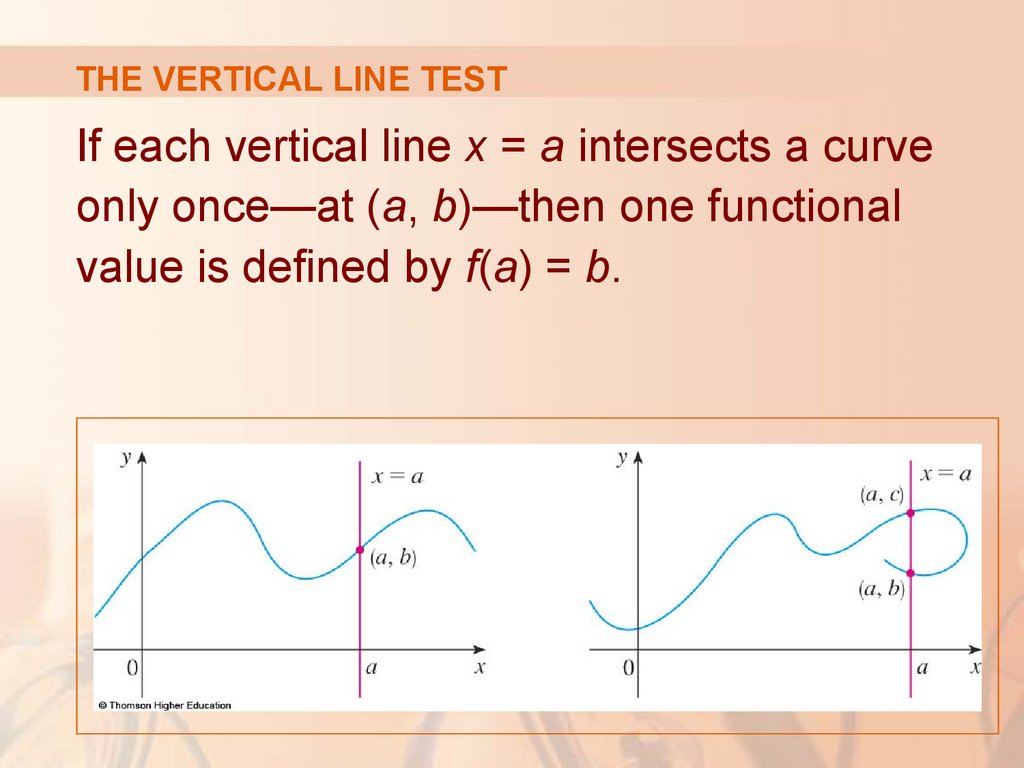
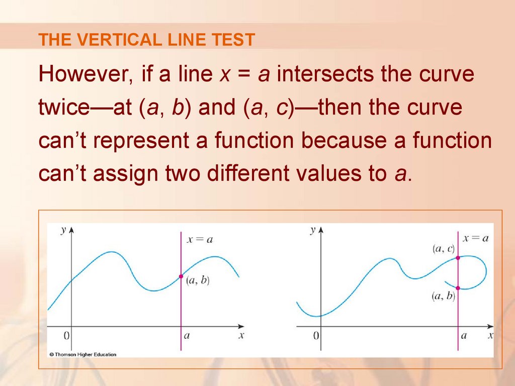
ground as measured by a seismograph
during an earthquake is a function of
the elapsed time t.

12.

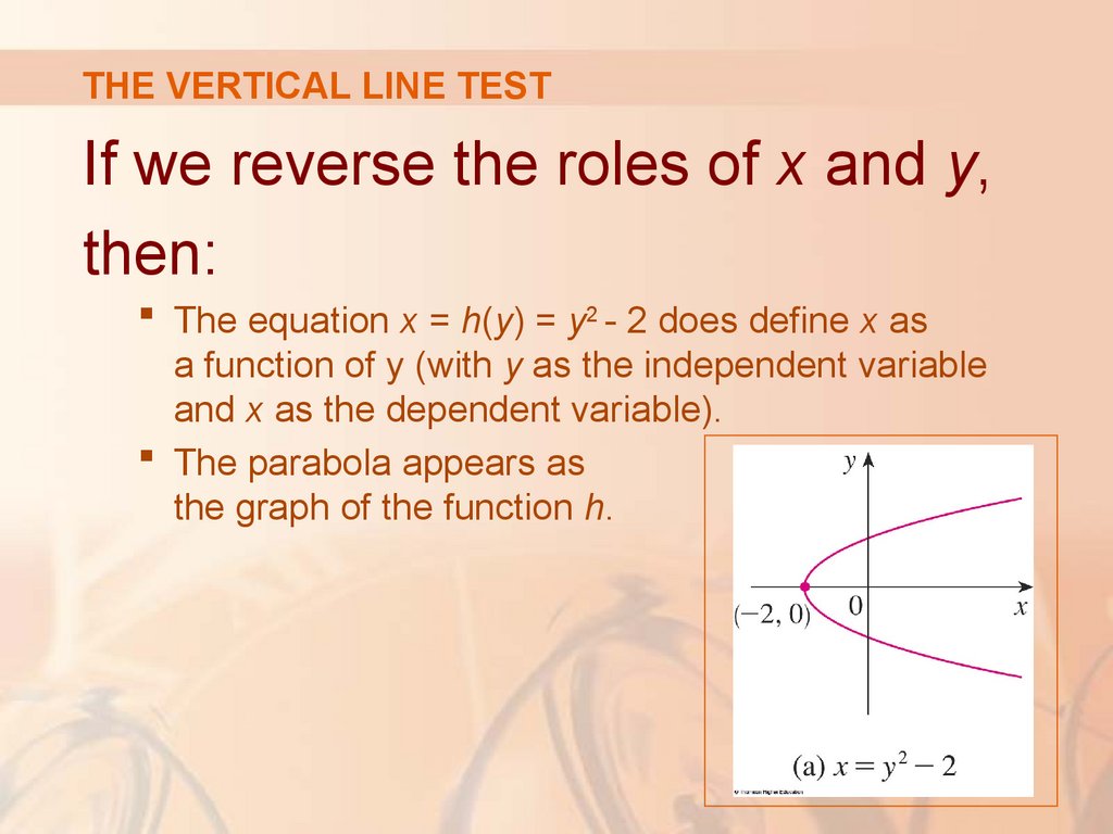
EXAMPLE D
The figure shows a graph generated by
seismic activity during the Northridge
earthquake that shook Los Angeles in
1994.
For a given value of t, the graph provides
a corresponding value of a.

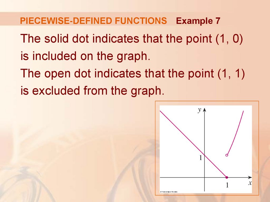
13.

FUNCTION
Each of these examples describes a rule
whereby, given a number (r, t, w, or t),
another number (A, P, C, or a) is
assigned.
In each case, we say that the second number
is a function of the first number.

14.

FUNCTION
A function f is a rule that assigns to
each element x in a set D exactly
one element, called f(x), in a set E.

15.

DOMAIN
We usually consider functions for
which the sets D and E are sets of
real numbers.
The set D is called the domain of the
function.

16.

VALUE AND RANGE
The number f(x) is the value of f at x
and is read ‘f of x.’
The range of f is the set of all possible
values of f(x) as x varies throughout the
domain.

17.

INDEPENDENT VARIABLE
A symbol that represents an arbitrary
number in the domain of a function f
is called an independent variable.
For instance, in Example A, r is the independent
variable.

18.

DEPENDENT VARIABLE
A symbol that represents a number in
the range of f is called a dependent
variable.
For instance, in Example A, A is the dependent variable.

19.

MACHINE
It’s helpful to think of a function
as a machine.
If x is in the domain of the function f, then when x
enters the machine, it’s accepted as an input and
the machine produces an output f(x) according to
the rule of the function.

20.

MACHINE
Thus, we can think of the domain as
the set of all possible inputs and the
range as the set of all possible
outputs.

21.

MACHINE
The preprogrammed functions in a
calculator are good examples of a
function as a machine.
For example, the square root key on your calculator
computes such a function.
You press the key labeled
(or x ) and enter
the input x.

22.

MACHINE
If x < 0, then x is not in the domain of this function
—that is, x is not an acceptable input,
and the calculator will indicate an error.
If x 0 , then an approximation to x will appear
in the display.
Thus, the x key on your calculator is not quite
the same as the exact mathematical function f
defined by f(x) = x .

23.

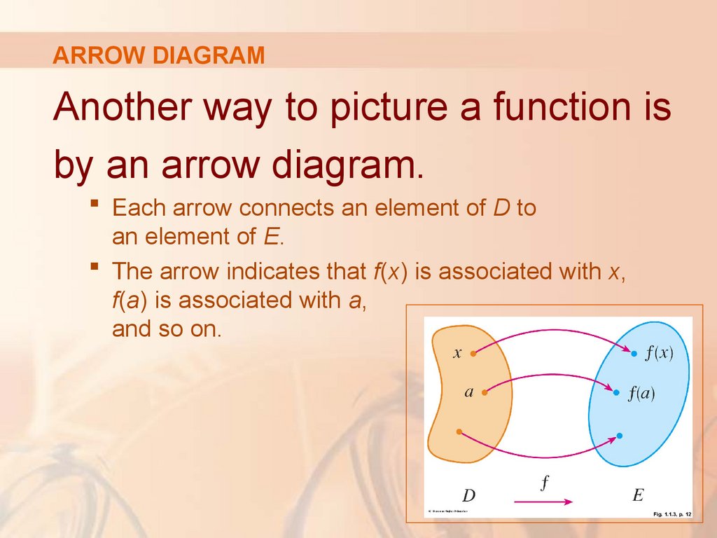
ARROW DIAGRAM
Another way to picture a function is
by an arrow diagram.
Each arrow connects an element of D to
an element of E.
The arrow indicates that f(x) is associated with x,
f(a) is associated with a,
and so on.
Fig. 1.1.3, p. 12

24.

GRAPH
The most common method for
visualizing a function is its graph.
If f is a function with domain D, then its graph is
the set of ordered pairs
( x, f ( x)) | x D
Notice that these are input-output pairs.
In other words, the graph of f consists of all points
(x, y) in the coordinate plane such that y = f(x)
and x is in the domain of f.

25.

GRAPH
The graph of a function f gives us
a useful picture of the behavior or
‘life history’ of a function.
Since the y-coordinate of any point (x, y) on
the graph is y = f(x), we can read the value of f(x)
from the graph as
being the height of
the graph above
the point x.

26.

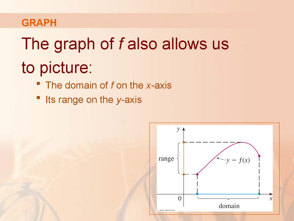
GRAPH
The graph of f also allows us
to picture:
The domain of f on the x-axis
Its range on the y-axis

27.

GRAPH
Example 1
The graph of a function f is shown.
a. Find the values of f(1) and f(5).
b. What is the domain and range of f ?

28.

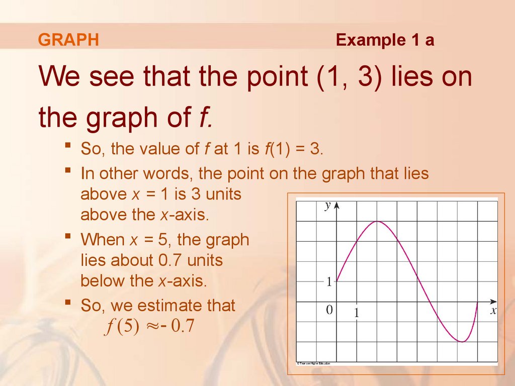
GRAPH
Example 1 a
We see that the point (1, 3) lies on
the graph of f.
So, the value of f at 1 is f(1) = 3.
In other words, the point on the graph that lies
above x = 1 is 3 units
above the x-axis.
When x = 5, the graph
lies about 0.7 units
below the x-axis.
So, we estimate that
f (5) 0.7

29.

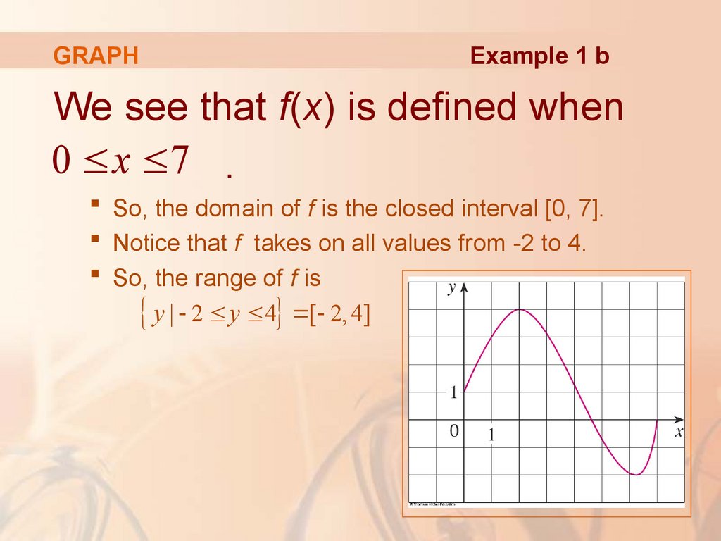
GRAPH
Example 1 b
We see that f(x) is defined when
0 x 7 .
So, the domain of f is the closed interval [0, 7].
Notice that f takes on all values from -2 to 4.
So, the range of f is
y | 2 y 4 [ 2, 4]

30.

GRAPH
Example 2
Sketch the graph and find the
domain and range of each function.
a. f(x) = 2x – 1
b. g(x) = x2

31.

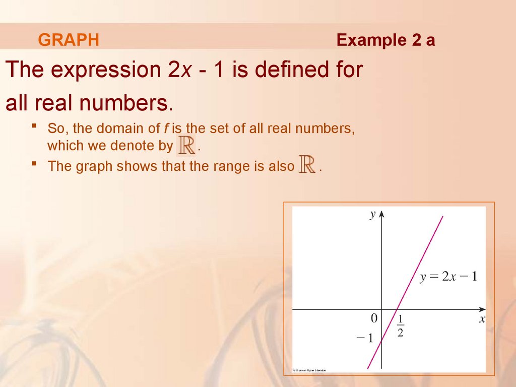
GRAPH
Example 2 a
The equation of the graph is:
y = 2x – 1
We recognize this as being the equation of a line
with slope 2 and y-intercept -1.
Recall the slope-intercept form of the equation of
a line: y = mx + b.
This enables us to sketch a portion of the graph of f,
as follows.

32.

GRAPH
Example 2 a
The expression 2x - 1 is defined for
all real numbers.
So, the domain of f is the set of all real numbers,
which we denote by
.
The graph shows that the range is also
.

33.

GRAPH
Example 2 b
Since g(2) = 22 = 4 and g(-1) = (-1)2 = 1,
we could plot the points (2, 4) and (-1, 1),
together with a few other points on the graph,
and join them to produce the next graph.

34.

GRAPH
Example 2 b
The equation of the graph is y = x2,
which represents a parabola.
The domain of g is .

35.

GRAPH
Example 2 b
The range of g consists of all values of
g(x), that is, all numbers of the form x2.
However, x 2 0 for all numbers x, and any positive
number y is a square.
So, the range of g is
y | y 0 [0, )
This can also be seen
from the figure.

36.

FUNCTIONS
Example 3
2
If f ( x) 2 x 5 x 1 and h 0 ,
evaluate:
f (a h) f (a )
h

37.

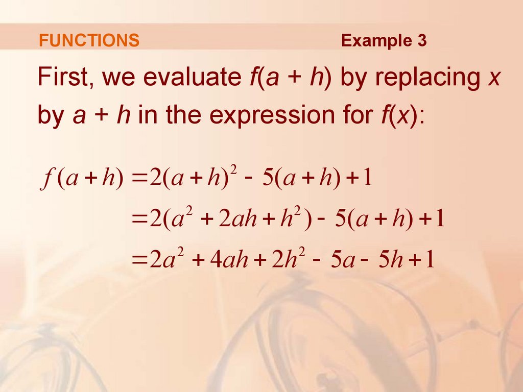
FUNCTIONS
Example 3
First, we evaluate f(a + h) by replacing x
by a + h in the expression for f(x):
2
f (a h) 2(a h) 5(a h) 1
2(a 2 2ah h 2 ) 5(a h) 1
2
2
2a 4ah 2h 5a 5h 1

38.

FUNCTIONS
Example 3
Then, we substitute it into the given
expression and simplify:
f (a h) f (a )
h
2
2
2
(2a 4ah 2h 5a 5h 1) (2a 5a 1)
h
2a 2 4ah 2h 2 5a 5h 1 2a 2 5a 1
h
4ah 2h 2 5h
4a 2h 5
h

39.

REPRESENTATIONS OF FUNCTIONS
There are four possible ways to
represent a function:
Verbally (by a description in words)
Numerically (by a table of values)
Visually (by a graph)
Algebraically (by an explicit formula)

40.

REPRESENTATIONS OF FUNCTIONS
If a single function can be represented
in all four ways, it’s often useful to go
from one representation to another to
gain additional insight into the function.
For instance, in Example 2, we started with
algebraic formulas and then obtained the graphs.

41.

REPRESENTATIONS OF FUNCTIONS
However, certain functions are
described more naturally by one
method than by another.
With this in mind, let’s reexamine the four situations
that we considered at the beginning of this section.

42.

SITUATION A
The most useful representation of
the area of a circle as a function of
its radius is probably the algebraic
2
formula A(r ) r .
However, it is possible to compile a table of values
or to sketch a graph (half a parabola).
As a circle has to have a positive radius, the domain
is r | r 0 (0, ) , and the range is also (0, ).

43.

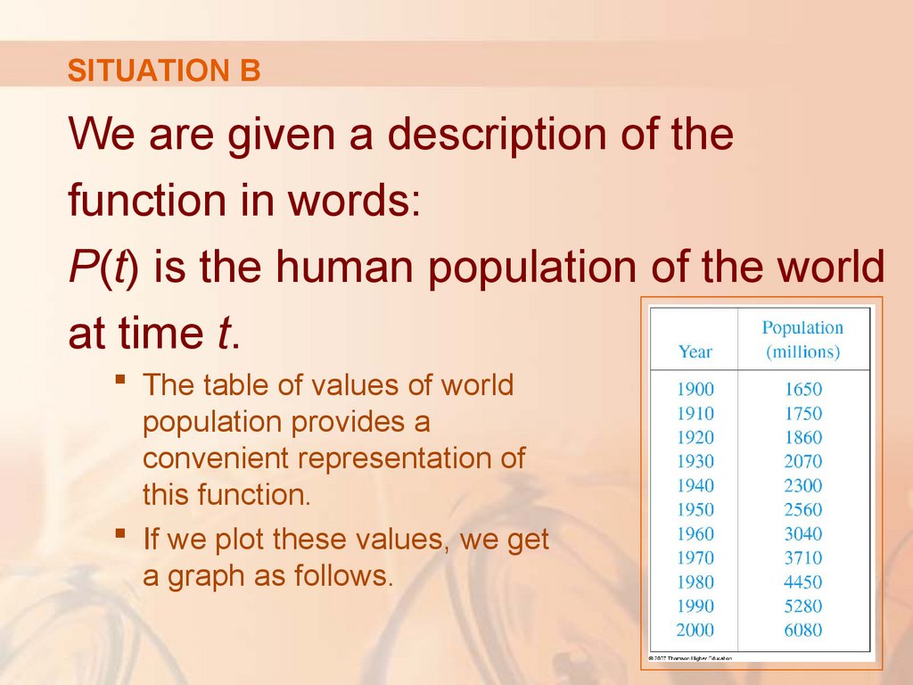
SITUATION B
We are given a description of the
function in words:
P(t) is the human population of the world
at time t.
The table of values of world
population provides a
convenient representation of
this function.
If we plot these values, we get
a graph as follows.

44.

SITUATION B
This graph is called a scatter plot.
It too is a useful representation.
It allows us to absorb all the data at once.

45.

SITUATION B
What about a formula?
Of course, it’s impossible to devise an explicit formula
that gives the exact human population P(t) at any time t.
However, it is possible to find an expression for
a function that approximates P(t).

46.

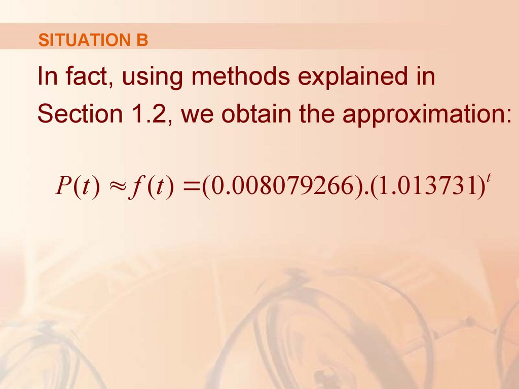
SITUATION B
In fact, using methods explained in
Section 1.2, we obtain the approximation:
P (t ) f (t ) (0.008079266).(1.013731)
t

47.

SITUATION B
This figure shows that the
approximation is a reasonably
good ‘fit.’

48.

SITUATION B
The function f is called a mathematical
model for population growth.
In other words, it is a function with an explicit
formula that approximates the behavior of our
given function.
However, we will see that the ideas of calculus
can be applied to a table of values.
An explicit formula is not necessary.

49.

SITUATION B
The function P is typical of the functions
that arise whenever we attempt to apply
calculus to the real world.
We start with a verbal description of a function.
Then, we may be able to construct a table of values
of the function—perhaps from instrument readings
in a scientific experiment.

50.

SITUATION B
Even though we don’t have complete
knowledge of the values of the function,
we will see throughout the book that it is
still possible to perform the operations of
calculus on such a function.

51.

SITUATION C
Again, the function is described in
words:
C(w) is the cost of mailing a first-class letter with
weight w.
The rule that the US Postal Service
used as of 2006 is:
The cost is 39 cents for up to one ounce, plus 24 cents
for each successive ounce up to 13 ounces.

52.

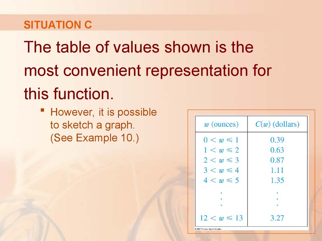
SITUATION C
The table of values shown is the
most convenient representation for
this function.
However, it is possible
to sketch a graph.
(See Example 10.)

53.

SITUATION D
The graph shown is the most
natural representation of the vertical
acceleration function a(t).

54.

SITUATION D
It’s true that a table of values could
be compiled.
It is even possible to devise an
approximate formula.

55.

SITUATION D
However, everything a geologist needs to
know—amplitudes and patterns—can be
seen easily from the graph.
The same is true for the patterns seen in
electrocardiograms of heart patients and polygraphs
for lie-detection.

56.

REPRESENTATIONS
In the next example, we sketch the
graph of a function that is defined
verbally.

57.

REPRESENTATIONS
Example 4
When you turn on a hot-water faucet, the
temperature T of the water depends on how
long the water has been running.
Draw a rough graph of T as a function of
the time t that has elapsed since the faucet
was turned on.

58.

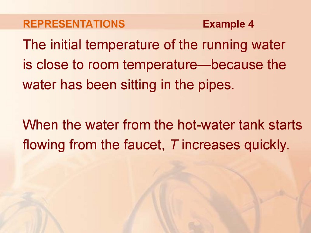
REPRESENTATIONS
Example 4
The initial temperature of the running water
is close to room temperature—because the
water has been sitting in the pipes.
When the water from the hot-water tank starts
flowing from the faucet, T increases quickly.

59.

REPRESENTATIONS
Example 4
In the next phase, T is constant at the
temperature of the heated water in the tank.
When the tank is drained, T decreases to
the temperature of the water supply.

60.

REPRESENTATIONS
Example 4
This enables us to make the rough
sketch of T as a function of t.

61.

REPRESENTATIONS
In the following example, we start with
a verbal description of a function in
a physical situation and obtain an explicit
algebraic formula.
The ability to do this is a useful skill in solving calculus
problems that ask for the maximum or minimum values
of quantities.

62.

REPRESENTATIONS
Example 5
A rectangular storage container with an
open top has a volume of 10 m3.
The length of its base is twice its width.
Material for the base costs $10 per square meter.
Material for the sides costs $6 per square meter.
Express the cost of materials as a
function of the width of the base.

63.

REPRESENTATIONS
Example 5
We draw a diagram and introduce notation—
by letting w and 2w be the width and length of
the base, respectively, and h be the height.

64.

REPRESENTATIONS
Example 5
The area of the base is (2w)w = 2w2.
So, the cost, in dollars, of the material
for the base is 10(2w2).

65.

REPRESENTATIONS
Example 5
Two of the sides have an area wh and
the other two have an area 2wh.
So, the cost of the material for the sides is
6[2(wh) + 2(2wh)].

66.

REPRESENTATIONS
Example 5
Therefore, the total cost is:
2
2
C 10(2 w ) 6[2( wh) 2(2 wh)] 20 w 36 wh

67.

REPRESENTATIONS
Example 5
To express C as a function of w alone,
we need to eliminate h.
We do so by using the fact that the
volume is 10 m3.
10
5
Thus, w(2 w) h 10 , which gives h 2 2
2w
w

68.

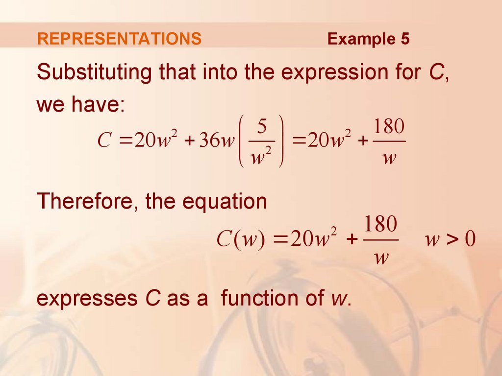
REPRESENTATIONS
Example 5
Substituting that into the expression for C,
we have:
180
5
2
2
C 20 w 36 w 2 20 w
w
w
Therefore, the equation
180
C ( w) 20 w
w
2
expresses C as a function of w.
w 0

69.

REPRESENTATIONS
Example 6
Find the domain of each function.
a. f ( x) x 2
1
b. g ( x) 2
x 1

70.

REPRESENTATIONS
Example 6 a
The square root of a negative number is
not defined (as a real number).
So, the domain of f consists of all values
of x such that x 2 0.
This is equivalent to x 2.
So, the domain is the interval [ 2, ) .

71.

REPRESENTATIONS
Example 6 b
1
1
Since g ( x) 2
x x x ( x 1)
and division by 0 is not allowed, we see
that g(x) is not defined when x = 0 or
x = 1.
Thus, the domain of g is x | x 0, x 1 .
This could also be written in interval notation
as ( , 0) (0,1) (1, ) .

72.

REPRESENTATIONS
The graph of a function is a curve in
the xy-plane.
However, the question arises:
Which curves in the xy-plane are graphs of functions?

73.

THE VERTICAL LINE TEST
A curve in the xy-plane is the graph
of a function of x if and only if no
vertical line intersects the curve more
than once.

74.

THE VERTICAL LINE TEST
The reason for the truth of the Vertical
Line Test can be seen in the figure.

75.

THE VERTICAL LINE TEST
If each vertical line x = a intersects a curve
only once—at (a, b)—then one functional
value is defined by f(a) = b.

76.

THE VERTICAL LINE TEST
However, if a line x = a intersects the curve
twice—at (a, b) and (a, c)—then the curve
can’t represent a function because a function
can’t assign two different values to a.

77.

THE VERTICAL LINE TEST
For example, the parabola x = y2 – 2
shown in the figure is not the graph of
a function of x.
This is because there are
vertical lines that intersect
the parabola twice.
The parabola, however,
does contain the graphs
of two functions of x.

78.

THE VERTICAL LINE TEST
Notice that the equation x = y2 - 2
implies y2 = x + 2, so y x 2
So, the upper and lower halves of the parabola
are the graphs of the functions f ( x) x 2
and g ( x) x 2

79.

THE VERTICAL LINE TEST
If we reverse the roles of x and y,
then:
The equation x = h(y) = y2 - 2 does define x as
a function of y (with y as the independent variable
and x as the dependent variable).
The parabola appears as
the graph of the function h.

80.

PIECEWISE-DEFINED FUNCTIONS
The functions in the following four
examples are defined by different formulas
in different parts of their domains.

81.

PIECEWISE-DEFINED FUNCTIONS Example 7
A function f is defined by:
1 x if x 1
f ( x) 2
if x 1
x
Evaluate f(0), f(1), and f(2) and
sketch the graph.

82.

PIECEWISE-DEFINED FUNCTIONS Example 7
Remember that a function is a rule.
For this particular function, the rule is:
First, look at the value of the input x.
If it happens that x 1, then the value of f(x) is 1 - x.
In contrast, if x > 1, then the value of f(x) is x2.

83.

PIECEWISE-DEFINED FUNCTIONS Example 7
Thus,
Since 0 1, we have f(0) = 1 - 0 = 1.
Since 1 1, we have f(1) = 1 - 1 = 0.
Since 2 > 1, we have f(2) = 22 = 4.

84.

PIECEWISE-DEFINED FUNCTIONS Example 7
How do we draw the graph of f ?
If x 1 , then f(x) = 1 – x.
So, the part of the graph of f that lies to the left of
the vertical line x = 1 must coincide with the line
y = 1 - x, which has slope -1 and y-intercept 1.
If x > 1, then f(x) = x2.
So, the part of the graph of f that lies to the right of
the line x = 1 must coincide with the graph of y = x2,
which is a parabola.
This enables us to sketch the graph as follows.

85.

PIECEWISE-DEFINED FUNCTIONS Example 7
The solid dot indicates that the point (1, 0)
is included on the graph.
The open dot indicates that the point (1, 1)
is excluded from the graph.

86.

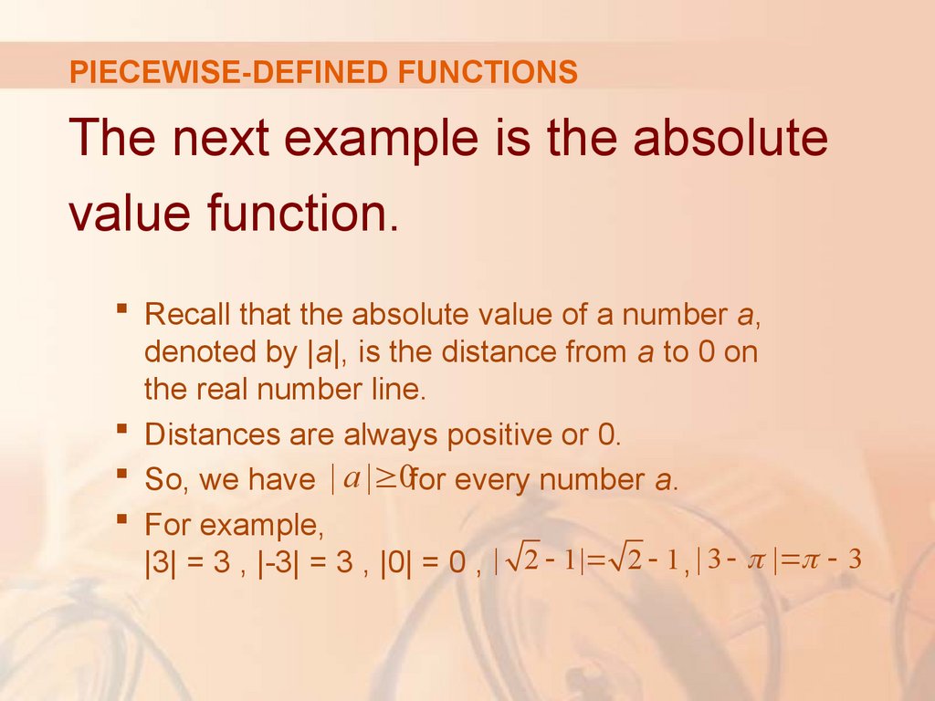
PIECEWISE-DEFINED FUNCTIONS
The next example is the absolute
value function.
Recall that the absolute value of a number a,
denoted by |a|, is the distance from a to 0 on
the real number line.
Distances are always positive or 0.
So, we have | a | 0for every number a.
For example,
|3| = 3 , |-3| = 3 , |0| = 0 , | 2 1| 2 1 , | 3 | 3

87.

PIECEWISE-DEFINED FUNCTIONS
In general, we have:
| a | a
if a 0
| a | a if a 0
Remember that, if a is negative, then -a is positive.

88.

PIECEWISE-DEFINED FUNCTIONS Example 8
Sketch the graph of the absolute
value function f(x) = |x|.
From the preceding discussion,
we know that:
if x 0
x
| x |
x if x 0

89.

PIECEWISE-DEFINED FUNCTIONS Example 8
Using the same method as in
Example 7, we see that the graph of f
coincides with:
The line y = x to the right of the y-axis
The line y = -x to the left of the y-axis

90.

PIECEWISE-DEFINED FUNCTIONS Example 9
Find a formula for the function f
graphed in the figure.

91.

PIECEWISE-DEFINED FUNCTIONS Example 9
The line through (0, 0) and (1, 1) has slope
m = 1 and y-intercept b = 0.
So, its equation is y = x.
Thus, for the part of
the graph of f that
joins (0, 0) to (1, 1),
we have:
f ( x) x if 0 x 1

92.

PIECEWISE-DEFINED FUNCTIONS Example 9
The line through (1, 1) and (2, 0) has slope
m = -1.
So, its point-slope form is y – 0 = (-1)(x - 2) or
y = 2 – x.
So, we have:
f ( x) 2 x if 1 x 2

93.

PIECEWISE-DEFINED FUNCTIONS Example 9
We also see that the graph of f coincides with
the x-axis for x > 2.
Putting this information together, we have
the following three-piece formula for f:
x
f ( x ) 2 x
0
if 0 x 1
if 1 x 2
if x 2

94.

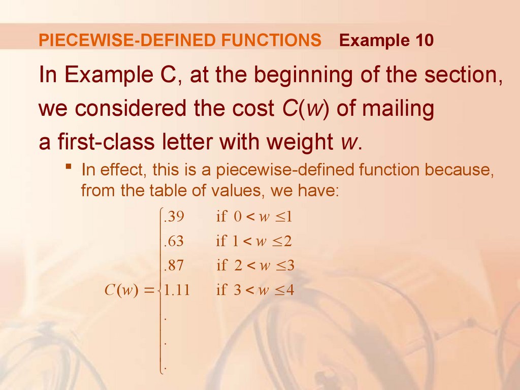
PIECEWISE-DEFINED FUNCTIONS Example 10
In Example C, at the beginning of the section,
we considered the cost C(w) of mailing
a first-class letter with weight w.
In effect, this is a piecewise-defined function because,
from the table of values, we have:
.39
.63
.87
C ( w) 1.11
.
.
.
if 0 w 1
if 1 w 2
if 2 w 3
if 3 w 4

95.

PIECEWISE-DEFINED FUNCTIONS Example 10
The graph is shown here.
You can see why functions like this are called
step functions—they jump from one value
to the next.
You will study such
functions in Chapter 2.

96.

SYMMETRY: EVEN FUNCTION
If a function f satisfies f(-x) = f(x) for
every number x in its domain, then f
is called an even function.
For instance, the function f(x) = x2 is even
because f(-x) = (-x)2 = x2 = f(x)

97.

SYMMETRY: EVEN FUNCTION
The geometric significance of an even
function is that its graph is symmetric with
respect to the y–axis.
This means that, if we
have plotted the graph of f
for x 0 , we obtain
the entire graph simply
by reflecting this portion
about the y-axis.

98.

SYMMETRY: ODD FUNCTION
If f satisfies f(-x) = -f(x) for every
number x in its domain, then f is called
an odd function.
For example, the function f(x) = x3 is odd
because f(-x) = (-x)3 = -x3 = -f(x)

99.

SYMMETRY: ODD FUNCTION
The graph of an odd function is
symmetric about the origin.
If we already have the graph of f for x 0 ,
we can obtain the entire graph by rotating
this portion through 180° about the origin.

100.

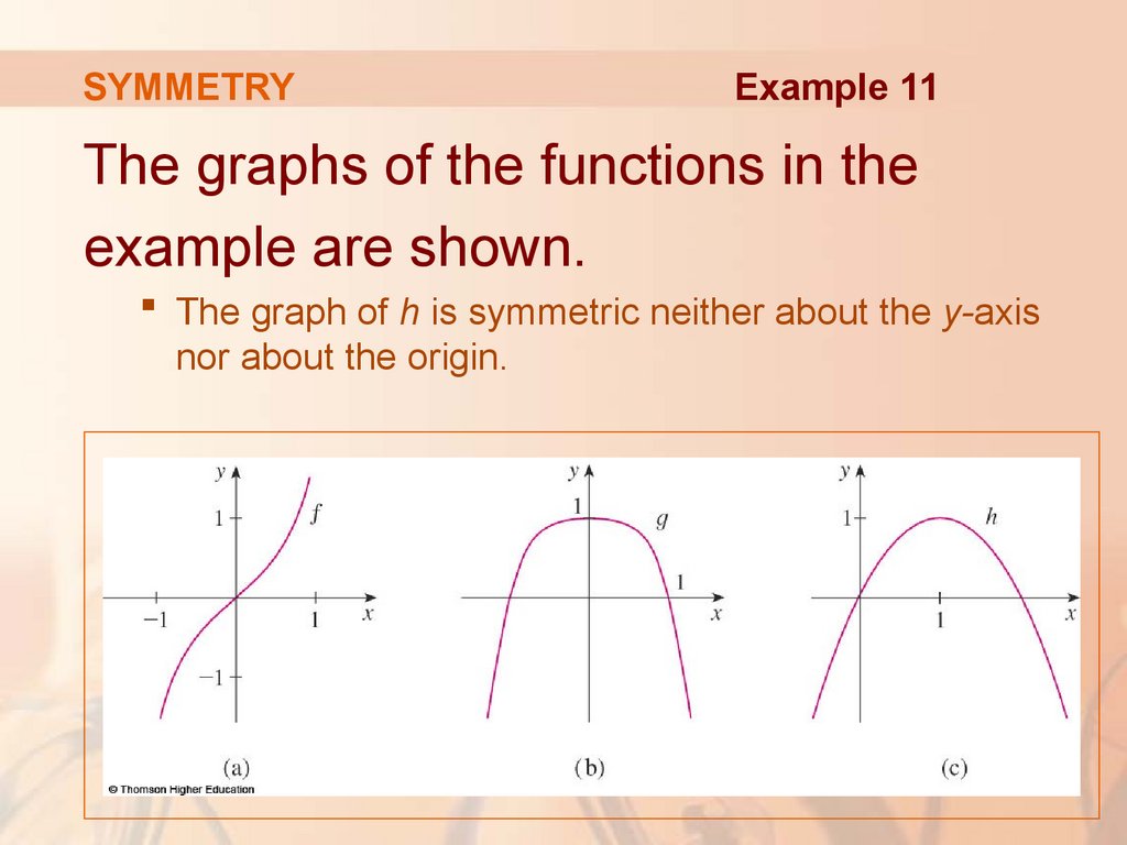
SYMMETRY
Example 11
Determine whether each of these functions
is even, odd, or neither even nor odd.
a. f(x) = x5 + x
b. g(x) = 1 - x4
c. h(x) = 2x - x2

101.

SYMMETRY
Example 11 a
5
5
5
f ( x) ( x) ( x) ( 1) x ( x)
5
5
x x ( x x )
f ( x)
Thus, f is an odd function.

102.

SYMMETRY
Example 11 b
4
4
g ( x) 1 ( x ) 1 x g ( x)
So, g is even.

103.

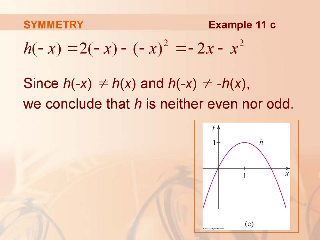
SYMMETRY
Example 11 c
2
h( x) 2( x) ( x) 2 x x
2
Since h(-x) h(x) and h(-x) -h(x),
we conclude that h is neither even nor odd.

104.

SYMMETRY
Example 11
The graphs of the functions in the
example are shown.
The graph of h is symmetric neither about the y-axis
nor about the origin.

105.

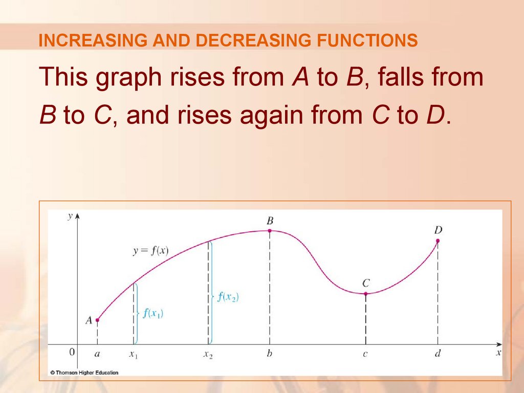
INCREASING AND DECREASING FUNCTIONS
This graph rises from A to B, falls from
B to C, and rises again from C to D.

106.

INCREASING AND DECREASING FUNCTIONS
The function f is said to be increasing on
the interval [a, b], decreasing on [b, c], and
increasing again on [c, d].

107.

INCREASING AND DECREASING FUNCTIONS
Notice that, if x1and x2 are any two numbers
between a and b with x1 < x2, then f(x1) < f(x2).
We use this as the defining property of
an increasing function.

108.

INCREASING AND DECREASING FUNCTIONS
A function f is called increasing on
an interval I if:
f(x1) < f(x2) whenever x1 < x2 in I
It is called decreasing on I if:
f(x1) > f(x2) whenever x1 < x2 in I

109.

INCREASING FUNCTION
In the definition of an increasing function,
it is important to realize that the inequality
f(x1) < f(x2) must be satisfied for every pair of
numbers x1 and x2 in I with x1 < x2.

110.

INCREASING AND DECREASING FUNCTIONS
You can see from the figure that the function
f(x) = x2 is decreasing on the interval ( , 0]
and increasing on the interval [0, ) .