Introduction to Computer Vision Lab 2

1.

Introduction to Computer Vision
Lab 2
Fall 2024

2.

Agenda
-
Recap
Convolution
Practice:
-
Noise
Smoothing
Filters
Affine Operations
Fall 2024

3.

Let’s start from images
An image is a picture (generally a 2D
projection of a 3D scene) captured by a
sensor that should be:
-
Sampled as n x m matrix
Quantised so that each element in
the matrix is given an integer value
(e.g. uint8 format)
Can we completely recognize what is
pictured?
But what about machine?
Fall 2024

4.

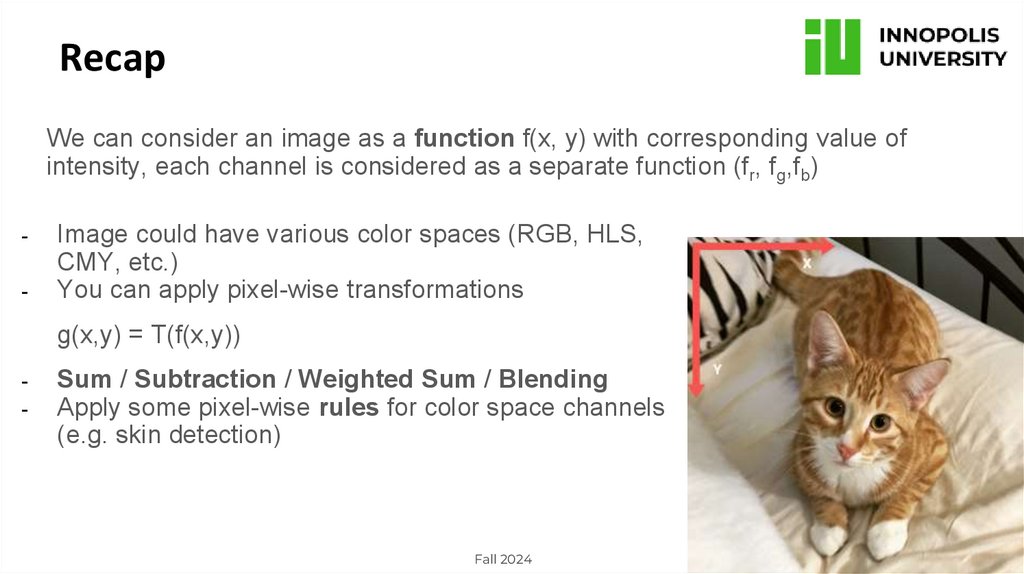
Recap
We can consider an image as a function f(x, y) with corresponding value of
intensity, each channel is considered as a separate function (fr, fg,fb)
-
Image could have various color spaces (RGB, HLS,
CMY, etc.)
You can apply pixel-wise transformations
g(x,y) = T(f(x,y))
-
Sum / Subtraction / Weighted Sum / Blending
Apply some pixel-wise rules for color space channels
(e.g. skin detection)
Fall 2024

5.

Let’s start with LSIS
We know that we are dealing with high-dimensional data like matrices meaning applying
some methods. But what properties these methods should follow?
Before we’re switching to more complex methods, somehow we should define them.
It turns out that in signal processing (CV in our case) is mainly focused on Linear ShiftInvariant Systems.
-
Linearity (System follows a superposition principle)
if f1 produces response g1(t) and f2(t) produces response g2(t), then any linear combination
a*f1(t) + b*f2(t) will produce the response a*g1(t) + b*g2(t), where a and b are constants.
-
Shift-Invariance (A shift-invariant system is one where a shift in the independent variable of the input
signal causes a corresponding shift in the output signal)
Fall 2024

6.

Linearity / Shift-Invariance graphically
In mathematics, a linear map or linear function f(x) is
a function that satisfies the two properties:
-
Additivity: f(x + y) = f(x) + f(y)
Homogeneity: f(αx) = α f(x) for all α
Homogeneity
superposition
Additivity
if we shift the input in time then the output is
shifted by the same amount.
if f(x(t)) = y(t), shift invariance means that f(x(t +
a)) = y(t + a).
Shift-Invariance
Fall 2024

7.

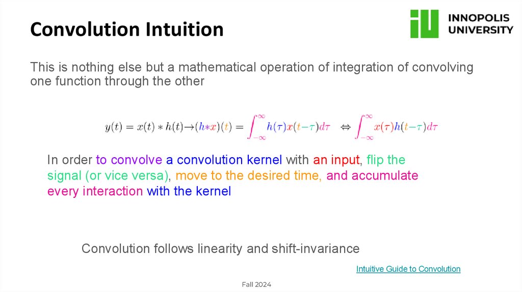
Convolution Intuition
This is nothing else but a mathematical operation of integration of convolving
one function through the other
In order to convolve a convolution kernel with an input, flip the
signal (or vice versa), move to the desired time, and accumulate
every interaction with the kernel
Convolution follows linearity and shift-invariance
Intuitive Guide to Convolution
Fall 2024

8.

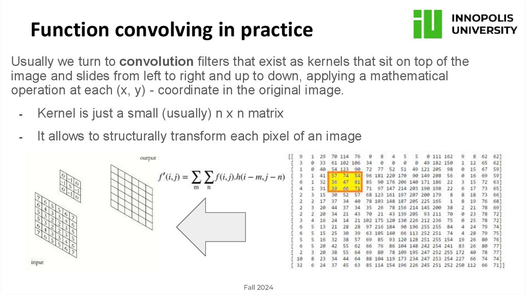
Function convolving in practice
Usually we turn to convolution filters that exist as kernels that sit on top of the
image and slides from left to right and up to down, applying a mathematical
operation at each (x, y) - coordinate in the original image.
-
Kernel is just a small (usually) n x n matrix
-
It allows to structurally transform each pixel of an image
Fall 2024

9.

Properties of convolution
-
Commutative → a * b = b * a
Associative → (a * b) * c = a * (b * c)
How does it help us?
If we are doing series of convolutions, then we can simplify our system
f → conv1 → conv2→ g ⇔ f → conv1 * conv2→ g ⇔ f → conv2* conv1→ g
Fall 2024

10.

Noise
Arise due to different reasons that distort
quality of our image
-
Gaussian Noise (good approximation for
real cases)
-
We need to identify it (measure) and
somehow correct it
-
Still we can evaluate it (practical problem?)
E.g. SSIM metric
Fall 2024

11.

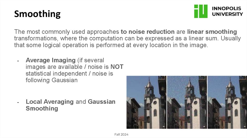
Smoothing
The most commonly used approaches to noise reduction are linear smoothing
transformations, where the computation can be expressed as a linear sum. Usually
that some logical operation is performed at every location in the image.
-
Average Imaging (if several
images are available / noise is NOT
statistical independent / noise is
following Gaussian
-
Local Averaging and Gaussian
Smoothing
Fall 2024

12.

One-image methods
If only one image exists, we still can apply techniques focused on pixel’s
neighbourhood by applying special filters. Simplest form is to compute local
average.
-
If points are equally weighted (h1) - we call this local averaging
Or we can define weights by some distribution - Gaussian (h2, h3)
Usually size of “fuzzy filter” is dependent upon the σ and kernel size
Median filter is better for edges preservation
BUT: we’re faced with blurring that
complicates an image processing
What exactly?
NOT every noise can be processed by
same methods. E.g. Median filter is best
suited for Salt & Pepper noise and the Wiener
filter can be used to remove the Speckle and
Poisson noise
Fall 2024

13.

Problem?
Great number of methods are computationally expensive - huge scope for
research.
-
Convolution → O(MNk2) for grayscale image
One way is to separate operations of filter itself (calculate separately for rows
and columns)
-
“Separable” convolution → O(2 * MNk)
Or change the principle. Example: Huang method (1979) or Perreault
approach (2007) for median filter.
However, specifically in this case histogram discretization IS NOT applicable
for a floating-point data (computed tomography)
Fall 2024

14.

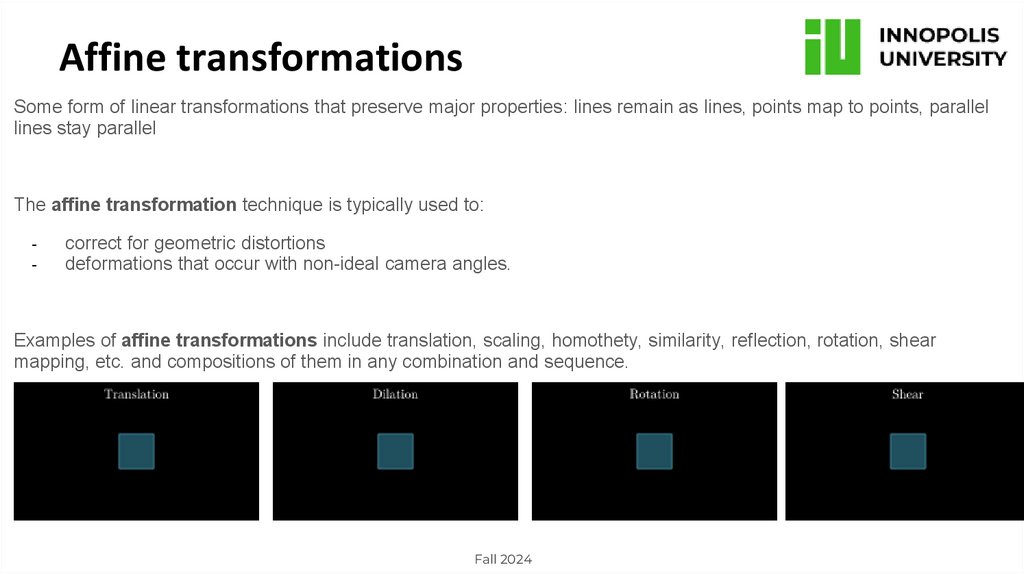
Affine transformations
Some form of linear transformations that preserve major properties: lines remain as lines, points map to points, parallel
lines stay parallel
The affine transformation technique is typically used to:
-
correct for geometric distortions
deformations that occur with non-ideal camera angles.
Examples of affine transformations include translation, scaling, homothety, similarity, reflection, rotation, shear
mapping, etc. and compositions of them in any combination and sequence.
Fall 2024

15.

That’s it
Next time …
Thresholding, Histograms, Image Gradients, Edge Detection and Morphological operations
Fall 2024