System reliability

1.

Performance evaluation:
Point of view Reliability
System reliability
Sofiene Dellagi
University of Metz /France
1

2. Definition

It’s the probability of successful operation of a system or
system component itself during a given time, reliability is a
dimension that is not the equivalent of "quantity", "value" of
the system considered. Corresponding to the degree of
confidence that can be placed in a machine or mechanism.
We note that reliability has become essential since the
equipment was complicated
Motivation
Failures in airplanes, rockets or nuclear plants quickly
become catastrophic; it is necessary to accurately predict the
uptime of each of these systems. Currently, this study is the
same time as the project construction
2

3. Definition and Notation

Reliability:
R(t) = Probability (S don’t fail on [0,t])
R(t) is a non increasing function varing between 1 à 0 on [0, +
Availability:
Availability A (t) is the probability that the system S is not in default at
time t. Note that in the case of non-repairable systems, the definition of
A (t) is equivalent to the reliability : A(t) = Probability (S is not default at
t)
Maintenability:
Maintainability M (t) :the probability that the system is repaired on the
interval [0 t] knowing that he has failed at time t = 0 :
M(t)=Probability (S is repaired on [0 t]/ S is failed at t=0 )
This concept applies only to repairable systems
M(t) is a non decreasing function varying between 0 à 1 on [0, +
3

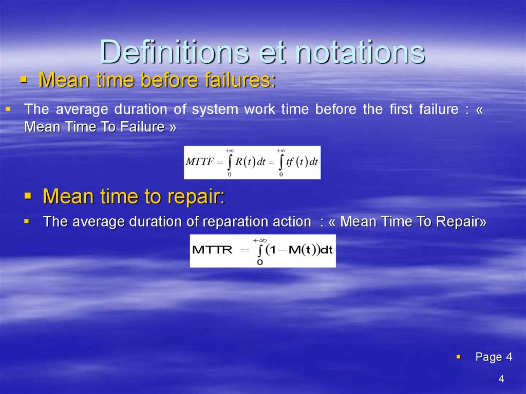
4. Definitions et notations

Mean time before failures:
The average duration of system work time before the first failure : «
Mean Time To Failure »
MTTF
0
0
R t dt tf t dt
Mean time to repair:
The average duration of reparation action : « Mean Time To Repair»
MTTR 1 M t dt
0
Page 4
4

5. Definitions et notations

Mean up time :
MUT:« Mean Up Time». It is different to MTTF because when the system is
returned to service after a failure, all breakdown elements have not
necessarily been repaired
Mean down time:
MDT:« Mean Down Time». This average corresponds to the detection of the
failure, duration of intervention, the duration of the repair and the ready time
Mean time between failure:
MTBF:« Mean Time Between Failure». Mean time between successive
failures
MTBF=MUT +MDT
MTTF MUT
5

6. stochastic Processes

Renewal process:
We consider a set of elements whose life is a continuous random
variable F with a probability density f. At time t = 0 is put into service the
first element and replaced by the following when a failure at time F1. If
Fr is the life of the r-th service element, its failure will occurs at date kr,
defined by: kr = F1 + F2 +….. Fr
We called renewal function the average value of the number of
rotation N (t) occurring on (0, t), the introduction of the first element at time t
= 0 is not counted as a renewal. H (t) = E [N (t)]
Called renewal density h (t) derivative H (t).
6

7. stochastic Processes

We called variable renewal process a renewal process for which
the random variable F1 has a different density than other random
variables Fi.
We Called residual life Vt the random variable representing the
remaining life of the item in service at time t
Page 25
26 27
7

8. Fondamental relations

We note by T the continuous random variable characterizing the
up time of the system
Re liabilityé:R t P T t
Failure fuction T: F t P T t 1 R t
F t failure probability on [0 t]
failure density : f t
dF t
dR t
dt
dt
Le temps moyen de bon fonctionnement:
MTTF
0
0
tf t dt R t dt
Mean time to repair : MTTR
1 M t dt
0
8

9. Relations fondamentales

Failure rate and repair rate
dR t
t
dt
R t exp u du
Failure rate t
R t
0
dM t
t
dt
M t 1 exp u du
repaire rate : t
1 M t
0
t
dR t
t R t t exp u du
failure density : f t
dt
0
t
dM t
t 1 M t t exp u du
Repair density :m t
dt
0
9

10. Method of determination of the material failure law « New material »

Method of determination of the
material failure law
« New material »
Experimentation
The Principe consists at making N new materials
working at t=0 assuring the same working
conditions.
10

11. Method of determination of the material failure law « New material »

Method of determination of the
material failure law
« New material »
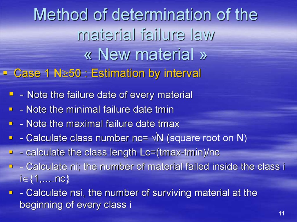
Case 1 N 50 : Estimation by interval
- Note the failure date of every material
- Note the minimal failure date tmin
- Note the maximal failure date tmax
- Calculate class number nc= N (square root on N)
- calculate the class length Lc=(tmax-tmin)/nc
- Calculate ni; the number of material failed inside the class i
i 1,….nc
- Calculate nsi, the number of surviving material at the
beginning of every class i
11

12. Method of determination of the material failure law « New material »

Method of determination of the
material failure law
« New material »
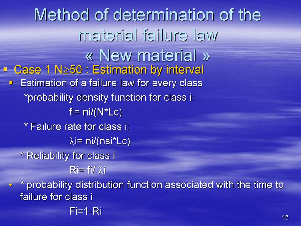
Case 1 N 50 : Estimation by interval
Estimation of a failure law for every class
*probability density function for class i:
fi= ni/(N*Lc)
* Failure rate for class i:
i= ni/(nsi*Lc)
* Reliability for class i
Ri= fi/ i
• * probability distribution function associated with the time to
failure for class i
Fi=1-Ri
12

13. Method of determination of the material failure law « New material »

Method of determination of the material
failure law
« New material »
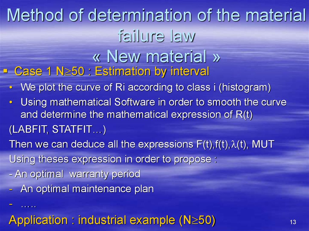
Case 1 N 50 : Estimation by interval
• We plot the curve of Ri according to class i (histogram)
• Using mathematical Software in order to smooth the curve
and determine the mathematical expression of R(t)
(LABFIT, STATFIT…)
Then we can deduce all the expressions F(t),f(t), (t), MUT
Using theses expression in order to propose :
- An optimal warranty period
- An optimal maintenance plan
- …..
Application : industrial example (N 50)
13

14. Method of determination of the material failure law « New material »

Method of determination of the
material failure law
« New material »
Case 2 N<50 : Punctual Estimation
- Note the failure date of every material
- classify the failure date by increasing order
(t1,t2,…….tN)
Let “i” representing the failure date order
For 20<N<50 (estimation by “rang moyen”)
• probability distribution function associated with the time to
failure according to ti:
Fi=i/(N+1)
14

15. Method of determination of the material failure law « New material »

Method of determination of the
material failure law
« New material »
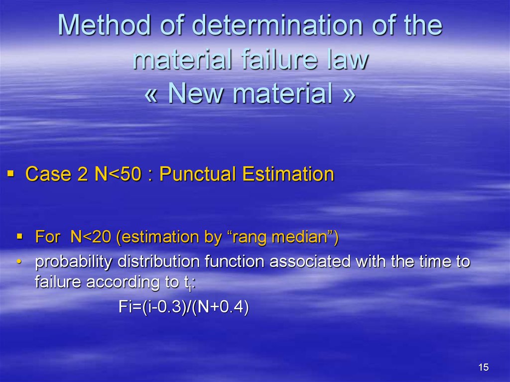
Case 2 N<50 : Punctual Estimation
For N<20 (estimation by “rang median”)
• probability distribution function associated with the time to
failure according to ti:
Fi=(i-0.3)/(N+0.4)
15

16. Method of determination of the material failure law « New material »

Method of determination of the
material failure law
« New material »
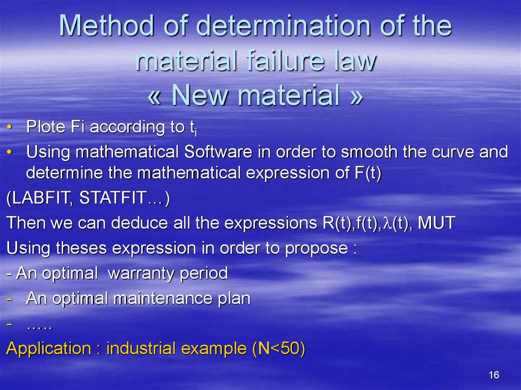
• Plote Fi according to ti
• Using mathematical Software in order to smooth the curve and
determine the mathematical expression of F(t)
(LABFIT, STATFIT…)
Then we can deduce all the expressions R(t),f(t), (t), MUT
Using theses expression in order to propose :
- An optimal warranty period
- An optimal maintenance plan
- …..
Application : industrial example (N<50)
16

17. Acceptance test for obtained law

Case 1 N 50 : KHI-Deux Test
• Compute E:
• E= ∑((ni-N*Pi)^2)/(N*Pi)
• And Pi= R(ti-1)-R(ti) with ti-1 and ti are respectively the born inf
and sup of every interval I
R is law obtained from the mathematical Software
• = nc-k-1 ( k the number of parameters of the considered law
• the value of the risk proposed by the industrial
• Note the value of ( , ) in the Khi-Deux table
• If E> ( , ) the law proposed is rejected
• If E ( , ) the law proposed is accepted
If the law is rejected we move to test another law
17

18. Acceptance test for obtained law

Case 2 N<50 : Klomorgov-Smirnov Test
• Compute D+ and D• D+ = max {(i/N)-F(ti)) , and D-= max F(ti)-((i-1)/N) ( i 1,2,..N
F is law obtained from the mathematical Software
• Compute D= max (D+, D-)
• the value of the risk proposed by the industrial
• Note the value of D ,N in the Klomorgov-Smirnov Table
• If D> D ,N the law proposed is rejected
• If D D ,N the law proposed is accepted
18

19. Principal law used in industry and research in reliability frame

19

20. Usuel discret law

20

21.

Dirac:
It’s a constant law
X a,
0
F x
1
si x a
si x a
E X a
V X 0
21

22.

Bernoulli:
1 si A
X 1A
0 si A
Parameter is p defined by p=P(A),
notation X →B(1,p)
X
F
E
V
1
0
0
q
1
x
X
X
p
q 1-p
si
x 0
si 0 x 1
si x 1
p
pq
p
1 p
Dem FIGURE
EXEMPLE page 66 67
22

23.

« binomiale »:
Parameters n and p=P(A)
PX X k
E X np
Cknpk
1 p
n_k
V X npq
Notation X →B(n,p)
Dem EXEMPLE page
69
23

24.

« Poisson » :
Parameters >0
PX X k e
E X
k
k!
V X
Notation
X →P( )
Dem EXEMPLE page
72 73 74
24

25.

« Pascal »:
Parameter k
AA
AA
k 1
Si on pose p P(A) la probabilité de cette évènememnt est:
Pk X k 1 p
k 1
p
1
p
q
V X 2
p
E X
Dem page 74 75
25

26.

« binomiale négative »:
Parameters n and y
:
A
A.........
.
A
A
.........
AA
A
y 1
On a n - 1 réalis atio ns de l' évènement A au cours de
y - 1 premières épreuves et qui s e conclut par
l' évènement A. On déduit la probabilit é individuelle :
y n
1
Pk Y y C n
pn
y 1 1 p
E Y
V Y
n
p
nq
p2
Dem page 75
26

27. Continuous law

Dem page 77 78
27

28.

« Loi uniforme »
k si x [a,b]
f x
0 si non
1
x a , b
b a
0
x a
La fonction de répartition: F x
b a
1
La densité :f
x
L'espérance: E x
V x
b a
si x < a
si a x < b
si b x
a b
2
2
12
En particulier a=0 et b=1
La densité :f
x
1
0
x 0,1
sinon
La fonction de répartition: F
x
0
x
1
si x < 0
si 0 x < 1
si 1 x
1
2
1
12
L'espérance: E x
La variance: V x
28

29.

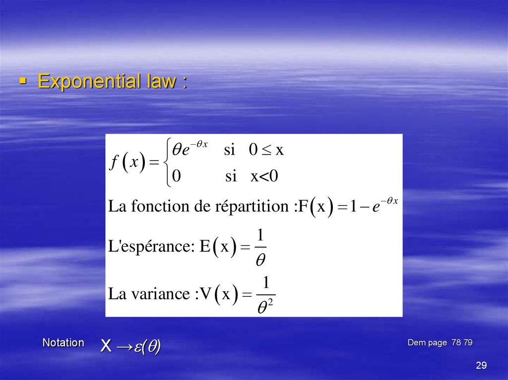
Exponential law :
e x si 0 x
f x
si x<0
0
La fonction de répartition :F x 1 e x
L'espérance: E x
La variance :V x
Notation
X → ( )
1
1
2
Dem page 78 79
29

30.

Laplace-Gauss:
Parameters m and
2
x m
1
f x
exp
2 2
2
L'espérance: E x m
La variance :V x 2
.Notation
X →N(m, )
Dem page 79 80-83
30

31.

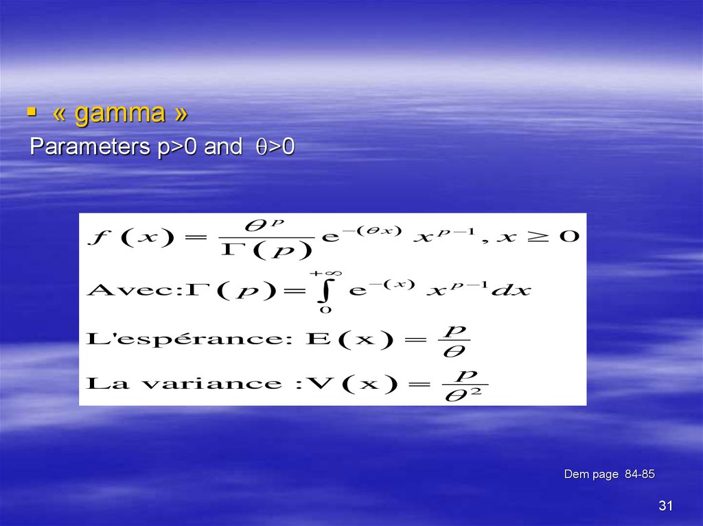
« gamma »
Parameters p>0 and >0
f
x
Avec:
p
p
p =
e x x
+
p 1
e x x
, x 0
p 1
dx
0
L'espérance: E
x
La variance :V
x
p
p
2
Dem page 84-85
31

32. Lois usuelles continues

« Khi-Deux »:
Gamma with p=n/2 and =1/2 ( (n/2, 1/2))
f
x
1
2
n
2
n
2
L'espérance: E
La variance :V
e
x
2
2
n
2
n
x
n
1
2
,x 0
n / 2
n
1/ 2
n / 2
2n
1/ 4
Dem page 85 86
32

33.

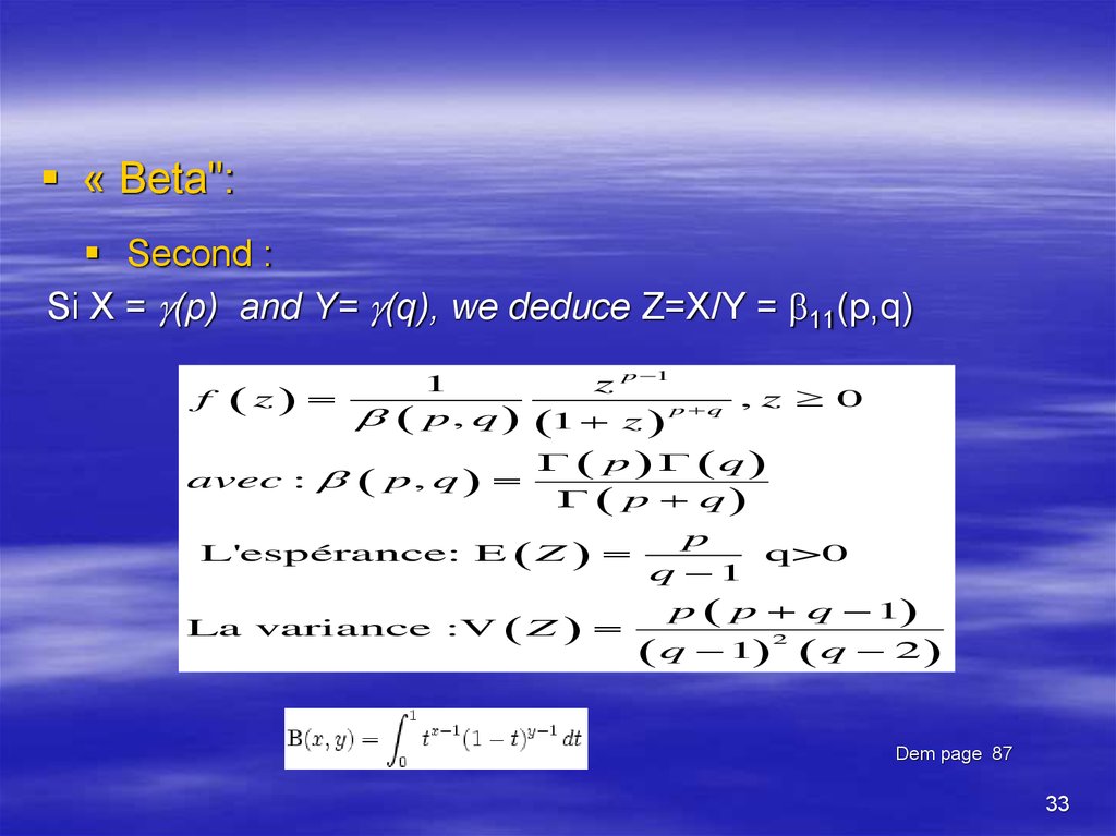
« Beta":
Second :
Si X = (p) and Y= (q), we deduce Z=X/Y = 11(p,q)
f
z
avec :
1
p, q
p, q
z
p 1
,z 0
1 z
p q
p q
L'espérance: E Z
La variance :V Z
p q
p
q>0
q 1
p p q 1
q
1
2
q
2
Dem page 87
33

34.

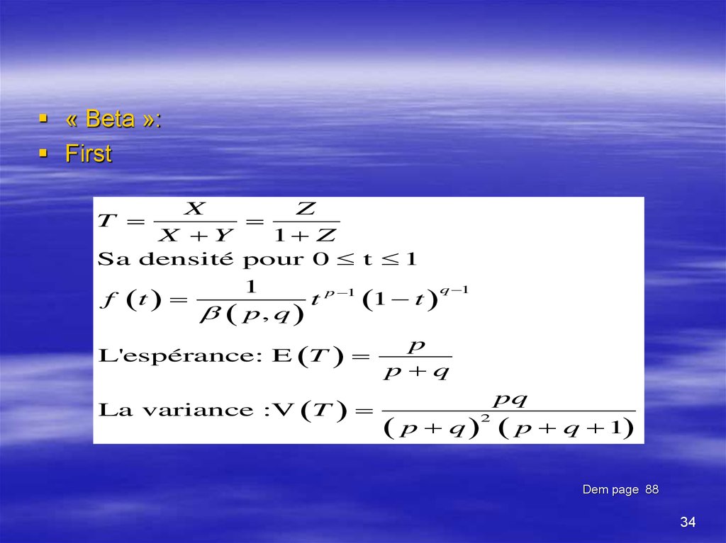
« Beta »:
First
X
Z
X Y
1 Z
Sa densité pour 0 t 1
T
f
t
1
q 1
t p 1 1 t
p, q
L'espérance: E T
La variance :V T
p
p q
pq
p q p q 1
2
Dem page 88
34

35.

« log-normale »:
Parameters m and
ln x m
La fonction de répartition: F x
1 ln x m
1
2
1
La densité est:f x
exp
ln
x
m
2
x x 2
2
AVEC : x
1
2
x
e
2
E ( X ) exp m
2
u2
2
V ( X ) exp 2m 2 exp 2 1
Dem page 90
35

36.

« Pareto »:
Parameters x0 (x x0>0) and >0:
La densité est:f x
1
x0
x0 x
x0
E X
avec >1
1
x0 2
V X
avec >2
2
1 2
Dem page 91
36

37. Lois Weibull trois paramètres

Densité de probabilité :
x
f ( x; , , )
( 1)
e
Fonction de répartition :
F ( x; , , ) 1 e
x
x

38. Lois Weibull deux paramètres ( ,)

Lois Weibull deux paramètres ( , )
Densité de probabilité :
Fonction de répartition :
x
f ( x; , )
( 1)
F ( x; , ) 1 e
e
x
x

39.

Structures
series
Dem page 91
39

40.

Structures
parallel
Series-parallel
Parallel-series
Dem page 91
40

41.

Complex Structures
Bridge system
Theorem of Bays
Exampl
Dem page 91
41

42.

Structures
series
parallel
Parallel-series
Series-parallel
Dem page 91
42

43.

Structures
series
parallel
Parallel-series
Series-parallel
Dem page 91
43

44.

Thank you for attention
Dem page 91
44