Value at Risk

1.

Value at Risk

2. The Question Being Asked in VaR

“What loss level is such that we are X%
confident it will not be exceeded in N
business days?”

3. VaR and Regulatory Capital (Business Snapshot 18.1, page 436)

Regulators base the capital they require
banks to keep on VaR
The market-risk capital is k times the 10day 99% VaR where k is at least 3.0

4. VaR vs. C-VaR (See Figures 18.1 and 18.2)

VaR is the loss level that will not be
exceeded with a specified probability
C-VaR (or expected shortfall) is the
expected loss given that the loss is greater
than the VaR level
Although C-VaR is theoretically more
appealing, it is not widely used

5. Advantages of VaR

It captures an important aspect of risk
in a single number
It is easy to understand
It asks the simple question: “How bad can
things get?”

6. Time Horizon

Instead of calculating the 10-day, 99% VaR
directly analysts usually calculate a 1-day 99%
VaR and assume
10 - day VaR 10 1- day VaR
This is exactly true when portfolio changes on
successive days come from independent
identically distributed normal distributions

7. Historical Simulation (See Tables 18.1 and 18.2, page 438-439))

Create a database of the daily movements in all
market variables.
The first simulation trial assumes that the
percentage changes in all market variables are
as on the first day
The second simulation trial assumes that the
percentage changes in all market variables are
as on the second day
and so on

8. Historical Simulation continued

Suppose we use m days of historical data
Let vi be the value of a variable on day i
There are m-1 simulation trials
The ith trial assumes that the value of the
market variable tomorrow (i.e., on day m+1) is
vi
vm
vi 1

9. The Model-Building Approach

The main alternative to historical simulation is to
make assumptions about the probability
distributions of return on the market variables
and calculate the probability distribution of the
change in the value of the portfolio analytically
This is known as the model building approach or
the variance-covariance approach

10. Daily Volatilities

In option pricing we measure volatility “per
year”
In VaR calculations we measure volatility
“per day”
day
year
252

11. Daily Volatility continued

Strictly speaking we should define day as
the standard deviation of the continuously
compounded return in one day
In practice we assume that it is the
standard deviation of the percentage
change in one day

12. Microsoft Example (page 440)

We have a position worth $10 million in
Microsoft shares
The volatility of Microsoft is 2% per day
(about 32% per year)
We use N=10 and X=99

13. Microsoft Example continued

The standard deviation of the change in
the portfolio in 1 day is $200,000
The standard deviation of the change in 10
days is
200,000 10 $632,456

14. Microsoft Example continued

We assume that the expected change in
the value of the portfolio is zero (This is
OK for short time periods)
We assume that the change in the value of
the portfolio is normally distributed
Since N(–2.33)=0.01, the VaR is
2.33 632,456 $1,473,621

15. AT&T Example (page 441)

AT&T Example (page 441)
Consider a position of $5 million in AT&T
The daily volatility of AT&T is 1% (approx
16% per year)
The S.D per 10 days is
50,000 10 $158,144
The VaR is
158,114 2.33 $368,405

16. Portfolio

Now consider a portfolio consisting of both
Microsoft and AT&T
Suppose that the correlation between the
returns is 0.3

17. S.D. of Portfolio

A standard result in statistics states that
X Y 2X Y2 2r X Y
In this case X = 200,000 and Y = 50,000
and r = 0.3. The standard deviation of the
change in the portfolio value in one day is
therefore 220,227

18. VaR for Portfolio

The 10-day 99% VaR for the portfolio is
220,227 10 2.33 $1,622,657
The benefits of diversification are
(1,473,621+368,405)–1,622,657=$219,369
What is the incremental effect of the AT&T
holding on VaR?
Options, Futures, and Other Derivatives 6th Edition, Copyright ©
18.18
John C.
Hull 2005

19.

20. Overview

Concepts
Components
Calculations
Corporate perspective
Comments

21.

I VALUE AT RISK - CONCEPTS

22. Risk

Financial Risks - Market Risk,
Credit Risk, Liquidity Risk,
Operational Risk
Risk is the variability of returns.
Risk is Defined as “Bad” Outcomes
Volatility Inappropriate Measure
What Matters is Downside Risk

23. VAR measures

Market risk
Credit risk of late

24. Value at Risk (VAR)

VAR is an estimate of the adverse impact on P&L in a
conservative scenario.
It is defined as the loss that can be sustained on a
specified position over a specified period with a
specified degree of confidence.

25. Value at Risk (VAR)

Ingredients
Exposure to market variable
Sensitivity
Probability of adverse market movement
Probability distribution of market variable - key
assumption
Normal, Log-normal distribution

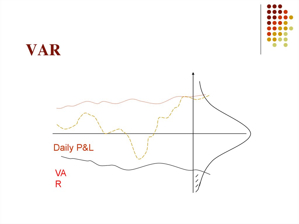
26. VAR

Daily P&L
VA
R

27.

VAR
Daily P&L
VA
R

28.

II VALUE AT RISK COMPONENTS

29. Key components of VAR

Market Factors (MF)
Factor Sensitivity (FS)
Defeasance Period (DP)
Volatility

30. Market Factors (MF)

A market variable that causes the price of an instrument
to change
A market factors group (MFG) is a group of market
factors with significant correlation. The major MFGs are:
Interest rates,
Foreign exchange rates
Equity prices
Commodity prices
Implied volatilities (only in options)
Complex positions can be sensitive to several MFG (e.g.
FX forwards or options)

31. Factor Sensitivity (FS)

FS is the change in the value of a position due to a
unit change in an independent market factor, all
other market factors, if applicable, remaining
constant.
Other names - PVBP

32. Factor Sensitivity - Zero Coupon Bond

What is the 1 BP FS of a $2,100 1-year zero
coupon bond? (assume market rate is 5%)
MTM Value = $2,100 / (1.05) = $2,000.00
MTM Value = $2,100 / (1.0501) = $1,999.81
FS = $1,999.81 - $2,000.00 = -$0.19

33. Market Volatility

Volatility is a measure of the dispersion of a market
variable against its mean or average. This dispersion is
called Standard Deviation.
Variance := average deviation of the mean for a
historical sample size
Standard deviation : Square Root of the variance
The market expresses volatility in terms of annualized
Standard Deviation (1SD)

34. Estimating Volatility

1. Historical data analysis
2. Judgmental
3. Implied (from options prices)

35. Defeasance period

This is defined as the time elapsed (normally
expressed in days) before a position can be
neutralized either by hedging or liquidating
Defeasance period incorporates liquidity risk
(for trading) in risk measurement
Other names - Holding Period, Time horizon

36. Defeasance Factor (DF)

DF is the total volatility over the defeasance
period
On the assumption that daily price changes are
independent variables (~ correlation zero),
volatility is scaled by the square root of time
DF = Daily 2.326 SD * sqrt (DP), or
DF = Market Volatility * 2.326 *sqrt (DP / 260)
DF = Annual 1SD * 2.326 * sqrt (DP/260)

37. VAR formula

z p t * FS
VAR =
Where:
z is the constant giving the appropriate one-tailed Confidence
Interval.
p is the annualized standard deviation of the portfolio’s return
t is the holding period horizon
FS Factor Sensitivity

38. VAR

Daily P&L
VA
R

39.

III VALUE AT RISK CALCULATIONS

40. Sample VAR Calculations

Let us consider the following positions:
Long EUR against the USD : $ 1 MM
Long JPY against the USD : $ 1 MM
Each of these positions has a factor sensitivity of
+10,000

41. Sample VAR Calculations

Annual volatility of DEM is 9%
Volatility for N days = annual volatility x SQRT(N/ T)
where T is the total number of trading days in a year
(260)
Therefore, 1 day volatility of DEM= 9 x SQRT (1/260)
= 0.56%
This is 1 ,
so, 2.326 = 2.326 x 0.56% = 1.30%

42. Sample VAR Calculations

Now, a 1% change has an impact of 10,000 (FS)
So, a 1.30% change will have an impact of
1.30 x 10,000 = 13,000
This represents the impact of a 2.326 SD change in
the market factor over a 1 day period
Thus, in 1 out of 100 days we may cross actual loss of
$ 13,000. Our Value at Risk (VAR) is $13,000 on this
position

43. Sample VAR Calculations

Similarly, for JPY, the annual volatility is 12%
The 1 day volatility = 12 x SQRT (1/260) = 0.74%
2.326 SD = 2.326 x 0.74 = 1.73%
Impact of a 1% change = 10,000 (FS)
So, impact of a 1.73% change = 17,310
Our VAR on this position is $ 17,310

44.

IV VALUE AT RISK FOR
CORPORATIONS

45. VAR FOR CORPORATIONS

Trading portfolios
Longer time horizons for close outs
Business risk as opposed to trading risk
Holding period, business time horizon
VAR as a percentage of Capital

46. VAR FOR CORPORATIONS

Identify market variables impacting business
Map income sensitivity to market variables - Scenario
analysis
Based on volatilities of market factors and their
correlations, arrive at a worst case scenario given the
degree of confidence
Worst case income projection - acceptable or not?
Hedge to reduce VAR

47. VAR FOR CORPORATIONS

Hedging tools
Forward FX
Currency swaps
Interest Rate swaps
Options on non-INR market variables
Commodity futures
Commodity derivatives

48.

V VALUE AT RISK- A FEW
COMMENTS

49. Significance of VAR

Applicable mainly to trading portfolios
Regulatory capital requirements
Provides senior executives with a simple and effective
way to monitor risk.
VAR incorporates portfolio effects.
Uses history to predict near term future.

50. VAR : A Few Comments

VAR does not represent the maximum loss
VAR does not represent the actual loss
It represents the potential loss associated with a
specified level of confidence. In this case, 99% over 1
day
Increased VAR represents increased risk, decrease in
VAR represents decrease in risk
VAR limit is related to revenue potential

51. Where to use VAR?

Macro measure. High level monitoring, managing, eg.
Regional level
Currently used mainly for trading limits.
Strategic planning - Allocation of resources
However..
Not an efficient day to day tool.
Components - FS, Market volatility, Defeasance period,
Correlations are all integral parts of trading strategy.

52. How to use Var

Stress Testing : * “worst case” scenario
* Multiple Stress Scenarios
* Should include not only price moves
In excess of 2SD, but also other
market events likely to adversely
affect business
Back Testing : Compares actual daily P&L movements
predicted variance of P&L

53. General Market Risk Issues

Integrity
- Rate Reasonability
- At Inception
- Revaluation
Model Certification
Control Mechanisms / Checks and Balances
Corporate Culture!

54. Review

Loss occurs only if rates move adversely to the position
The loss is proportional to the sensitivity of the position
The loss is proportional to size of the adverse
movement
Loss = FS multiplied by the adverse rate movement
We cannot limit adverse rate movements in the
marketplace
We can limit our sensitivity (P&L impact) with FSL
FSL should be set against potential adverse movement
Potential adverse movements estimated through
volatility