Geometric Modeling - Parametric Representation of Synthetic Curves

1.

Week 7: Geometric Modeling Parametric Representation of
Synthetic Curves
Spring 2018, AUA
Zeid, I., Mastering CAD/CAM, Chapter 6

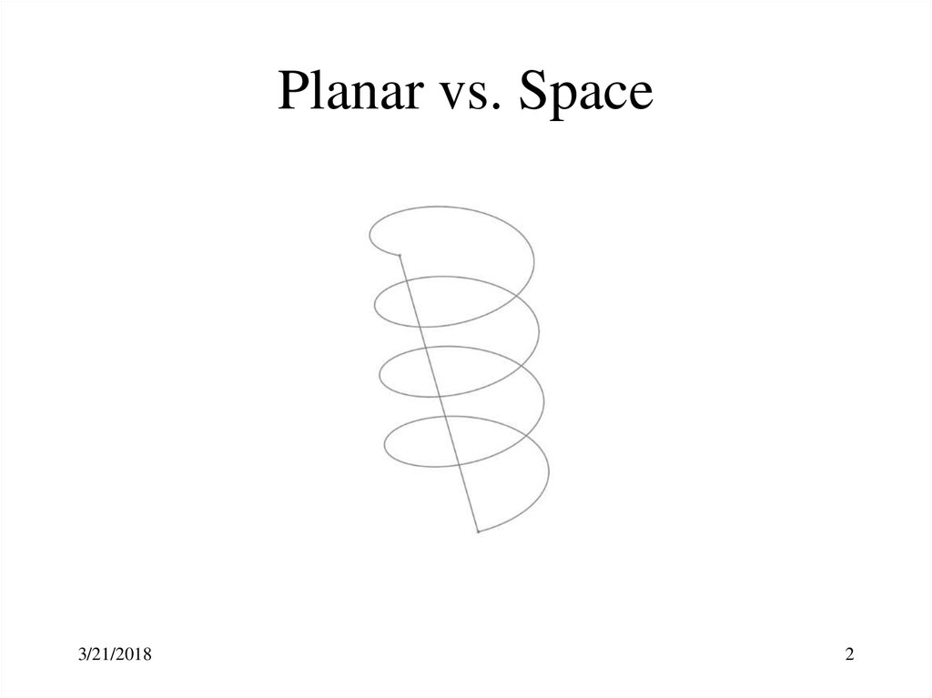
2. Planar vs. Space

3/21/2018
2

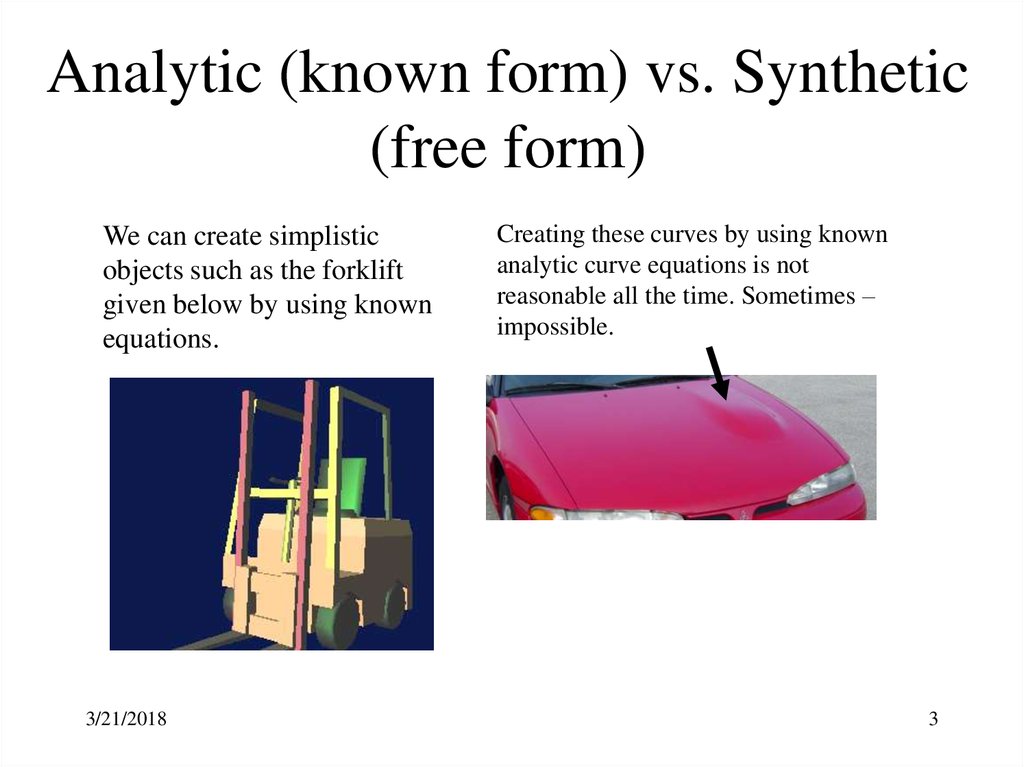
3. Analytic (known form) vs. Synthetic (free form)

We can create simplistic
objects such as the forklift
given below by using known
equations.
3/21/2018
Creating these curves by using known
analytic curve equations is not
reasonable all the time. Sometimes –
impossible.
3

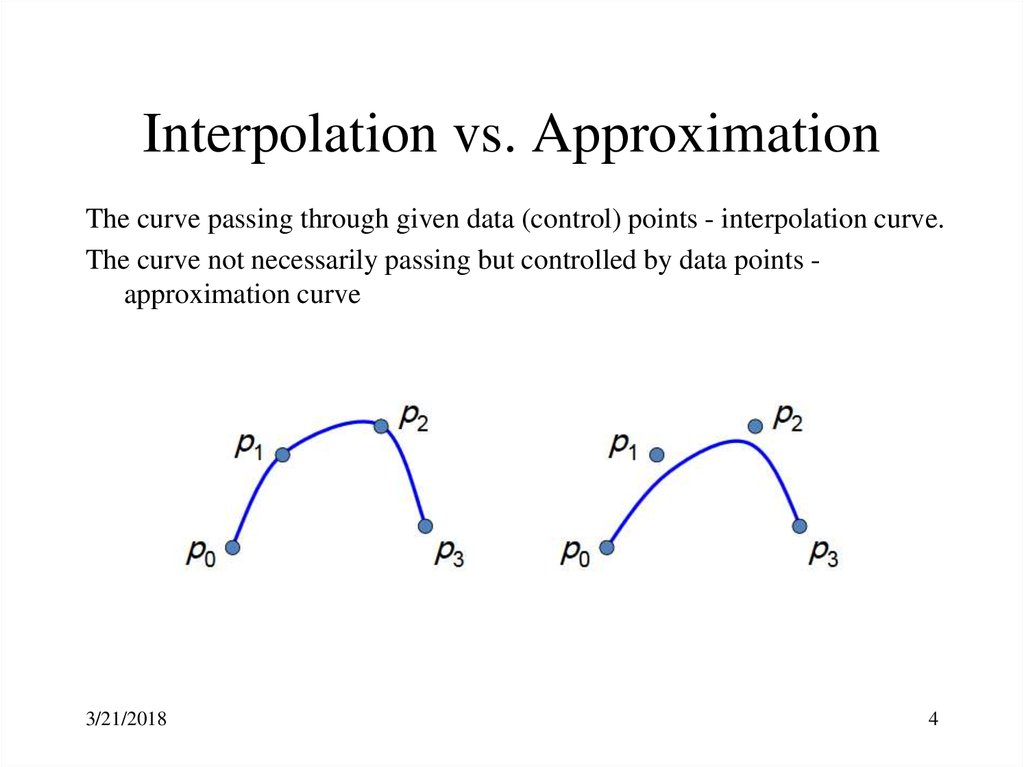
4. Interpolation vs. Approximation

The curve passing through given data (control) points - interpolation curve.
The curve not necessarily passing but controlled by data points approximation curve
3/21/2018
4

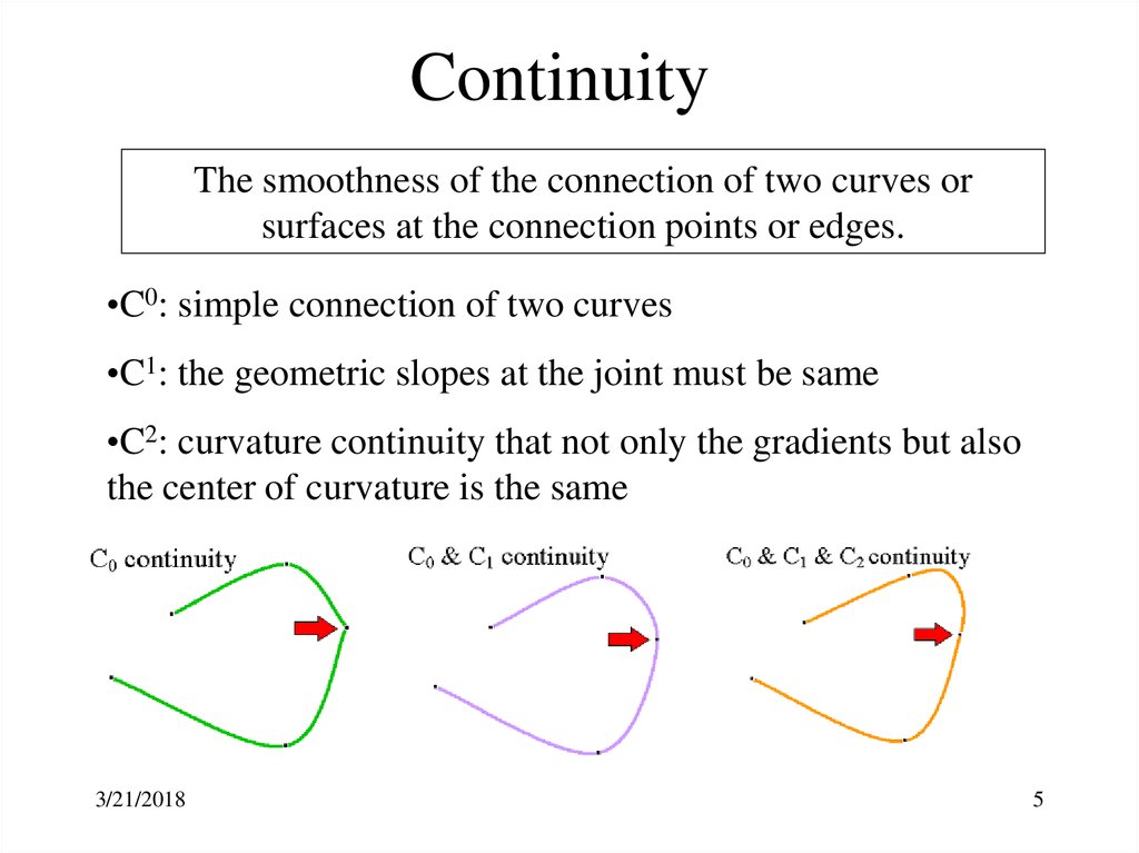
5. Continuity

The smoothness of the connection of two curves or
surfaces at the connection points or edges.
•C0: simple connection of two curves
•C1: the geometric slopes at the joint must be same
•C2: curvature continuity that not only the gradients but also
the center of curvature is the same
3/21/2018
5

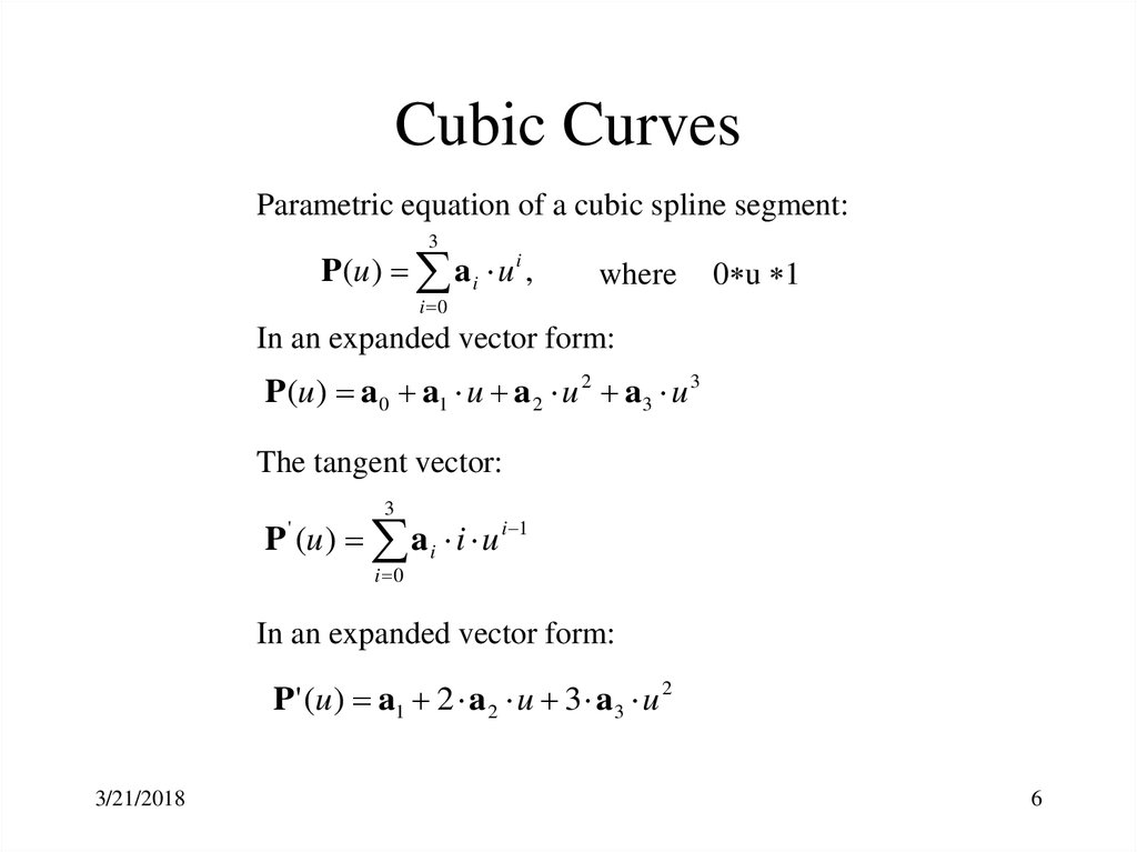
6. Cubic Curves

Parametric equation of a cubic spline segment:
3
P (u ) a i u i ,
where
0 u 1
i 0
In an expanded vector form:
P(u ) a 0 a1 u a 2 u 2 a 3 u 3
The tangent vector:
3
P (u ) a i i u i 1
'
i 0
In an expanded vector form:
P' (u ) a1 2 a 2 u 3 a 3 u 2
3/21/2018
6

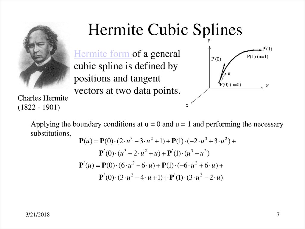
7. Hermite Cubic Splines

Charles Hermite
(1822 - 1901)
Hermite form of a general
cubic spline is defined by
positions and tangent
vectors at two data points.
P’(1)
P(1) (u=1)
P’(0)
tu
P(0) (u=0)
Applying the boundary conditions at u = 0 and u = 1 and performing the necessary
substitutions,
P(u ) P(0) (2 u 3 3 u 2 1) P(1) ( 2 u 3 3 u 2 )
P ' (0) (u 3 2 u 2 u ) P ' (1) (u 3 u 2 )
P ' (u ) P(0) (6 u 2 6 u ) P(1) ( 6 u 2 6 u )
P ' (0) (3 u 2 4 u 1) P ' (1) (3 u 2 2 u )
3/21/2018
7

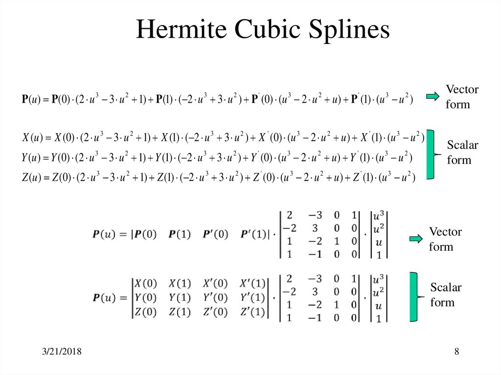
8. Hermite Cubic Splines

P(u ) P(0) (2 u 3 u 1) P(1) ( 2 u 3 u ) P (0) (u 2 u u ) P (1) (u u )
3
2
3
2
'
3
2
'
3
2
X (u ) X (0) (2 u 3 3 u 2 1) X (1) ( 2 u 3 3 u 2 ) X ' (0) (u 3 2 u 2 u ) X ' (1) (u 3 u 2 )
Y (u ) Y (0) (2 u 3 u 1) Y (1) ( 2 u 3 u ) Y (0) (u 2 u u ) Y (1) (u u )
3
2
3
2
'
3
2
'
3
2
Vector
form
Scalar
form
Z (u ) Z (0) (2 u 3 3 u 2 1) Z (1) ( 2 u 3 3 u 2 ) Z ' (0) (u 3 2 u 2 u ) Z ' (1) (u 3 u 2 )
Vector
form
Scalar
form
3/21/2018
8

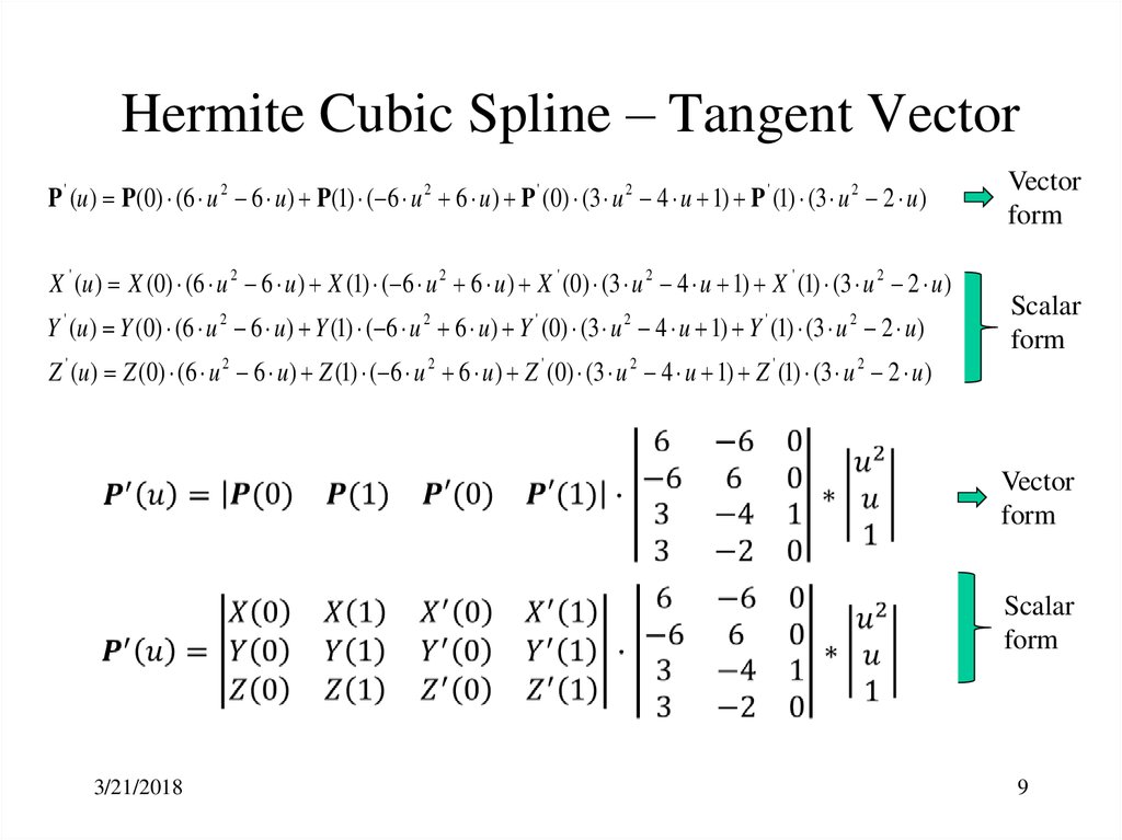
9. Hermite Cubic Spline – Tangent Vector

P ' (u ) P(0) (6 u 2 6 u ) P(1) ( 6 u 2 6 u ) P ' (0) (3 u 2 4 u 1) P ' (1) (3 u 2 2 u )
X ' (u ) X (0) (6 u 2 6 u ) X (1) ( 6 u 2 6 u ) X ' (0) (3 u 2 4 u 1) X ' (1) (3 u 2 2 u )
Y (u ) Y (0) (6 u 6 u ) Y (1) ( 6 u 6 u ) Y (0) (3 u 4 u 1) Y (1) (3 u 2 u )
'
2
2
'
2
'
2
Z ' (u ) Z (0) (6 u 2 6 u ) Z (1) ( 6 u 2 6 u ) Z ' (0) (3 u 2 4 u 1) Z ' (1) (3 u 2 2 u )
Vector
form
Scalar
form
Vector
form
Scalar
form
3/21/2018
9

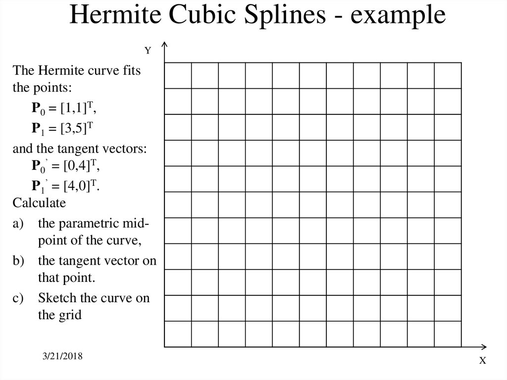
10. Hermite Cubic Splines - example

Y
The Hermite curve fits
the points:
P0 = [1,1]T,
P1 = [3,5]T
and the tangent vectors:
P0’ = [0,4]T,
P1’ = [4,0]T.
Calculate
a) the parametric midpoint of the curve,
b) the tangent vector on
that point.
c) Sketch the curve on
the grid
3/21/2018
X

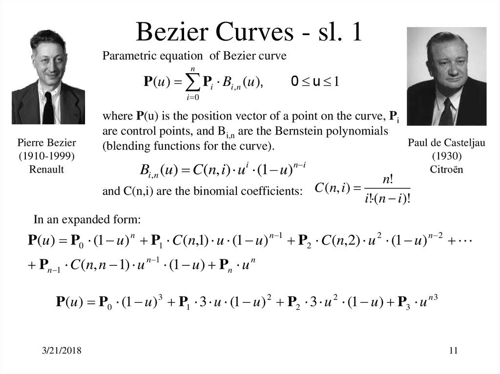
11. Bezier Curves - sl. 1

Parametric equation of Bezier curve
n
P(u ) Pi Bi ,n (u ),
0 u 1
i 0
Pierre Bezier
(1910-1999)
Renault
where P(u) is the position vector of a point on the curve, Pi
are control points, and Bi,n are the Bernstein polynomials
Paul de Casteljau
(blending functions for the curve).
Bi ,n (u) C(n, i) u (1 u)
i
n i
and C(n,i) are the binomial coefficients: C (n, i )
n!
i! (n i )!
(1930)
Citroën
In an expanded form:
P(u) P0 (1 u) n P1 C (n,1) u (1 u) n 1 P2 C (n,2) u 2 (1 u ) n 2
Pn 1 C (n, n 1) u n 1 (1 u) Pn u n
P(u ) P0 (1 u ) 3 P1 3 u (1 u ) 2 P2 3 u 2 (1 u ) P3 u n 3
3/21/2018
11

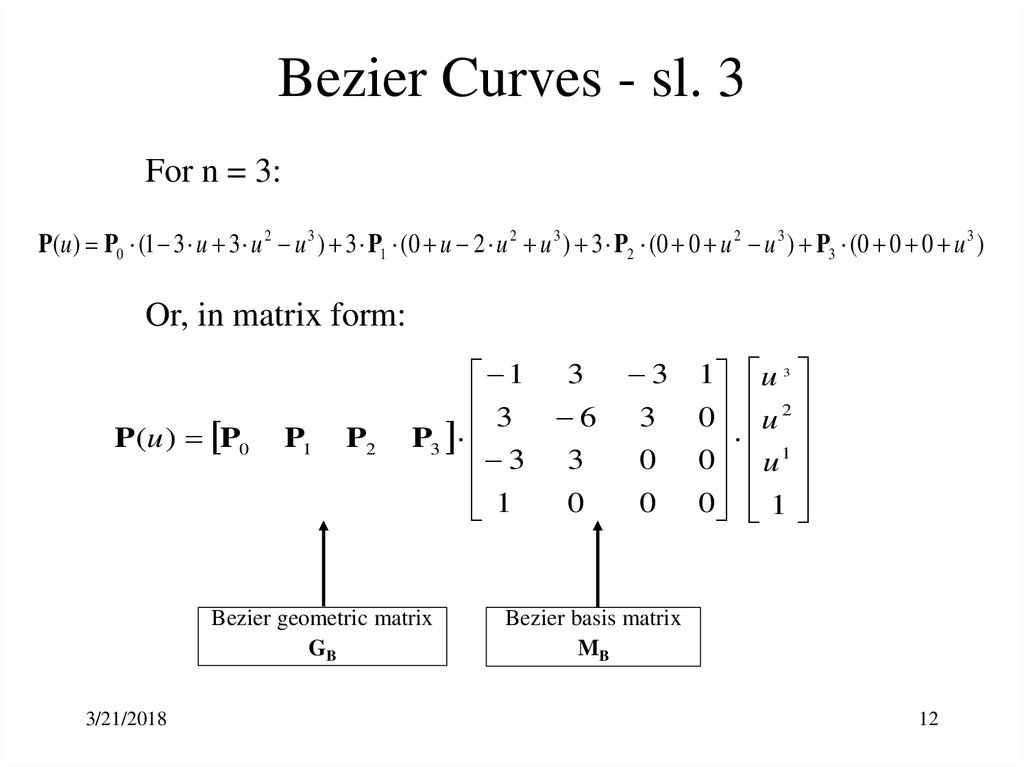
12. Bezier Curves - sl. 3

For n = 3:
P(u ) P0 (1 3 u 3 u 2 u 3 ) 3 P1 (0 u 2 u 2 u 3 ) 3 P2 (0 0 u 2 u 3 ) P3 (0 0 0 u 3 )
Or, in matrix form:
P (u ) P0
P1
P2
1
3
P3
3
1
Bezier geometric matrix
GB
3/21/2018
3
3
6
3
3
0
0
0
1 u 3
0 u 2
1
0 u
0 1
Bezier basis matrix
MB
12

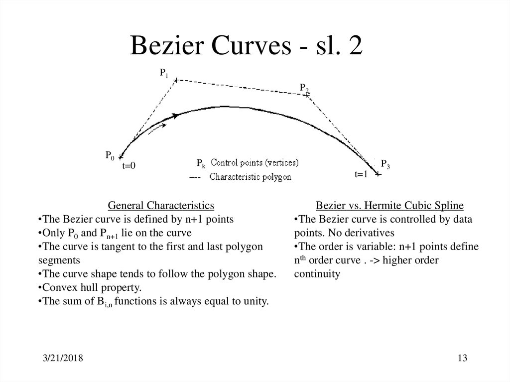
13. Bezier Curves - sl. 2

P1
P2
P0
t=0
Pk
General Characteristics
•The Bezier curve is defined by n+1 points
•Only P0 and Pn+1 lie on the curve
•The curve is tangent to the first and last polygon
segments
•The curve shape tends to follow the polygon shape.
•Convex hull property.
•The sum of Bi,n functions is always equal to unity.
3/21/2018
P3
t=1
Bezier vs. Hermite Cubic Spline
•The Bezier curve is controlled by data
points. No derivatives
•The order is variable: n+1 points define
nth order curve . -> higher order
continuity
13

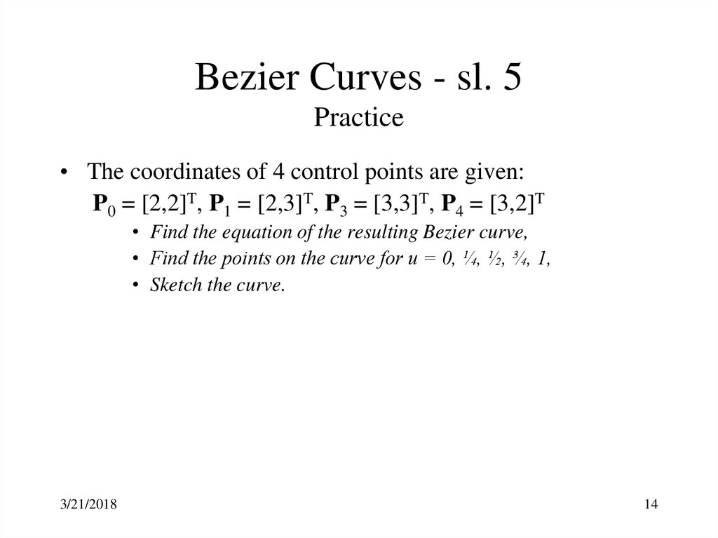
14. Bezier Curves - sl. 5 Practice

• The coordinates of 4 control points are given:
P0 = [2,2]T, P1 = [2,3]T, P3 = [3,3]T, P4 = [3,2]T
• Find the equation of the resulting Bezier curve,
• Find the points on the curve for u = 0, ¼, ½, ¾, 1,
• Sketch the curve.
3/21/2018
14

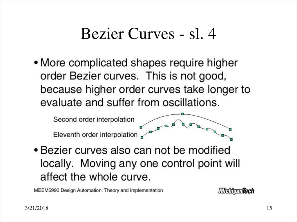
15. Bezier Curves - sl. 4

3/21/2018
15

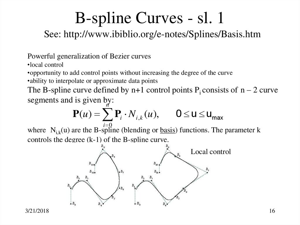
16. B-spline Curves - sl. 1 See: http://www.ibiblio.org/e-notes/Splines/Basis.htm

Powerful generalization of Bezier curves
•local control
•opportunity to add control points without increasing the degree of the curve
•ability to interpolate or approximate data points
The B-spline curve defined by n+1 control points Pi consists of n – 2 curve
segments and is given by:
n
P(u ) Pi N i ,k (u ),
i 0
0 u umax
where Ni,k(u) are the B-spline (blending or basis) functions. The parameter k
controls the degree (k-1) of the B-spline curve.
Local control
3/21/2018
16

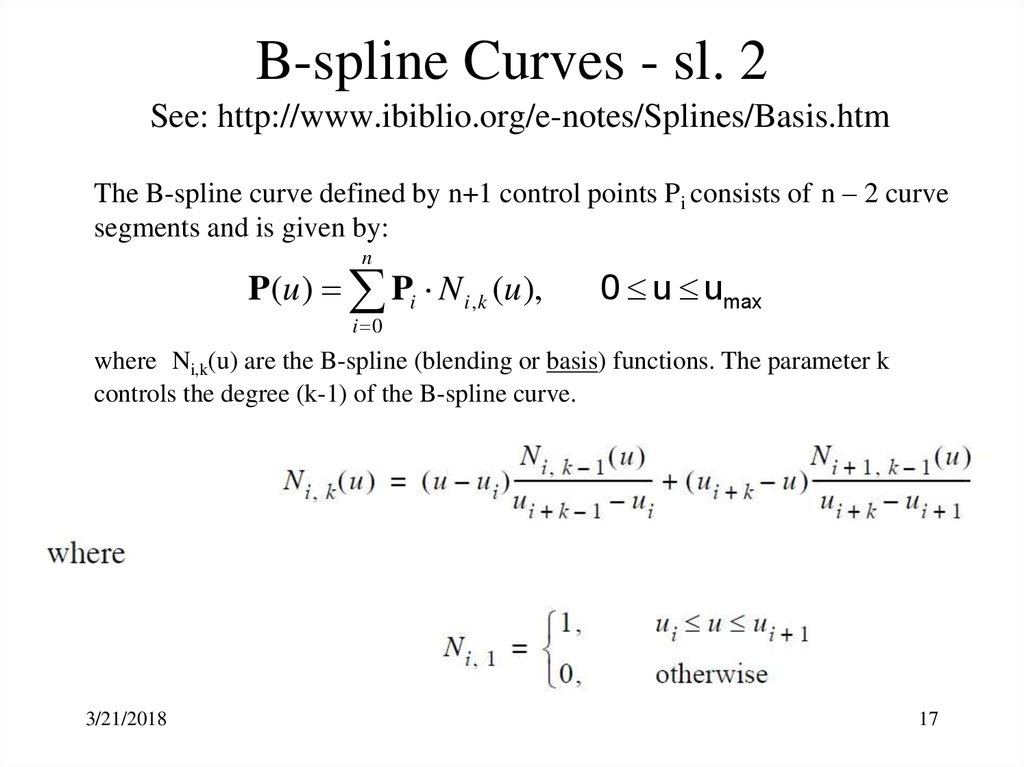
17. B-spline Curves - sl. 2 See: http://www.ibiblio.org/e-notes/Splines/Basis.htm

The B-spline curve defined by n+1 control points Pi consists of n – 2 curve
segments and is given by:
n
P(u ) Pi N i ,k (u ),
i 0
0 u umax
where Ni,k(u) are the B-spline (blending or basis) functions. The parameter k
controls the degree (k-1) of the B-spline curve.
3/21/2018
17

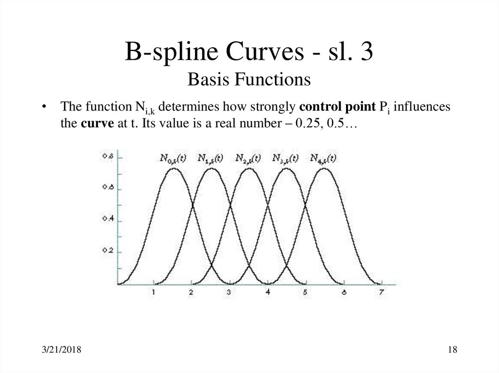
18. B-spline Curves - sl. 3 Basis Functions

• The function Ni,k determines how strongly control point Pi influences
the curve at t. Its value is a real number – 0.25, 0.5…
3/21/2018
18

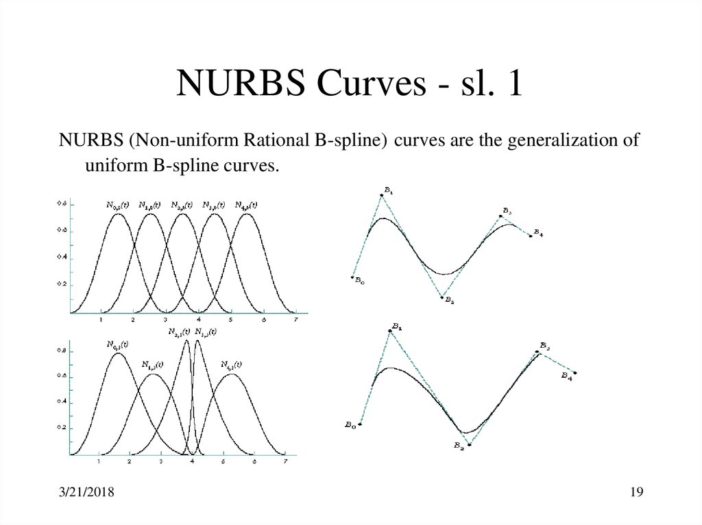
19. NURBS Curves - sl. 1

NURBS (Non-uniform Rational B-spline) curves are the generalization of
uniform B-spline curves.
3/21/2018
19

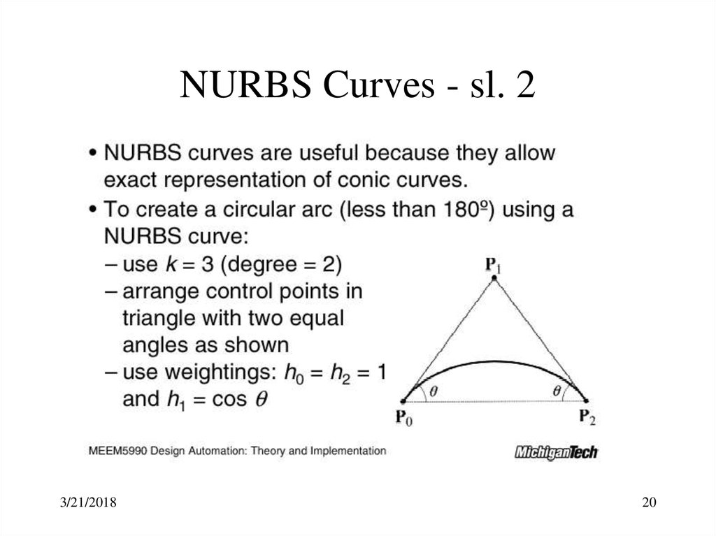
20. NURBS Curves - sl. 2

3/21/2018
20