Похожие презентации:
M&M: The Starting Point
1. Modigliani & Miller + WACC
Modigliani & Miller + WACC2. M&M: The Starting Point
M&M: The Starting PointA number of restrictive assumptions apply
Use the additivity principle
Derive propositions re: valuation and cost of
capital
Derived in both the “no tax” and “tax” cases.
FIN 591: Financial Fundamentals/Valuation
2
3. The M&M Assumptions
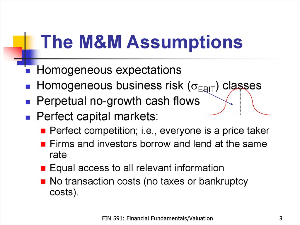
The M&M AssumptionsHomogeneous expectations
Homogeneous business risk (sEBIT) classes
Perpetual no-growth cash flows
Perfect capital markets:
Perfect competition; i.e., everyone is a price taker
Firms and investors borrow and lend at the same
rate
Equal access to all relevant information
No transaction costs (no taxes or bankruptcy
costs).
FIN 591: Financial Fundamentals/Valuation
3
4. Business Risk
Business risk:Risk surrounding expected operating cash flows
Factors causing high business risk:
High correlation between the firm and the economy
Firm has small market share in competitive market
Firm is small relative to competitors
Firm is not well diversified
Firm has high fixed operating costs.
FIN 591: Financial Fundamentals/Valuation
4
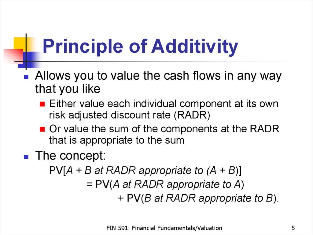
5. Principle of Additivity
Allows you to value the cash flows in any waythat you like
Either value each individual component at its own
risk adjusted discount rate (RADR)
Or value the sum of the components at the RADR
that is appropriate to the sum
The concept:
PV[A + B at RADR appropriate to (A + B)]
= PV(A at RADR appropriate to A)
+ PV(B at RADR appropriate to B).
FIN 591: Financial Fundamentals/Valuation
5
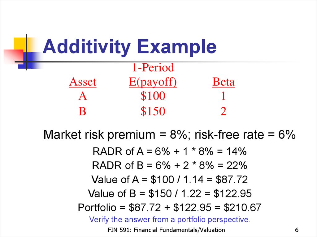
6. Additivity Example
AssetA
B
1-Period
E(payoff)
$100
$150
Beta
1
2
Market risk premium = 8%; risk-free rate = 6%
RADR of A = 6% + 1 * 8% = 14%
RADR of B = 6% + 2 * 8% = 22%
Value of A = $100 / 1.14 = $87.72
Value of B = $150 / 1.22 = $122.95
Portfolio = $87.72 + $122.95 = $210.67
Verify the answer from a portfolio perspective.
FIN 591: Financial Fundamentals/Valuation
6
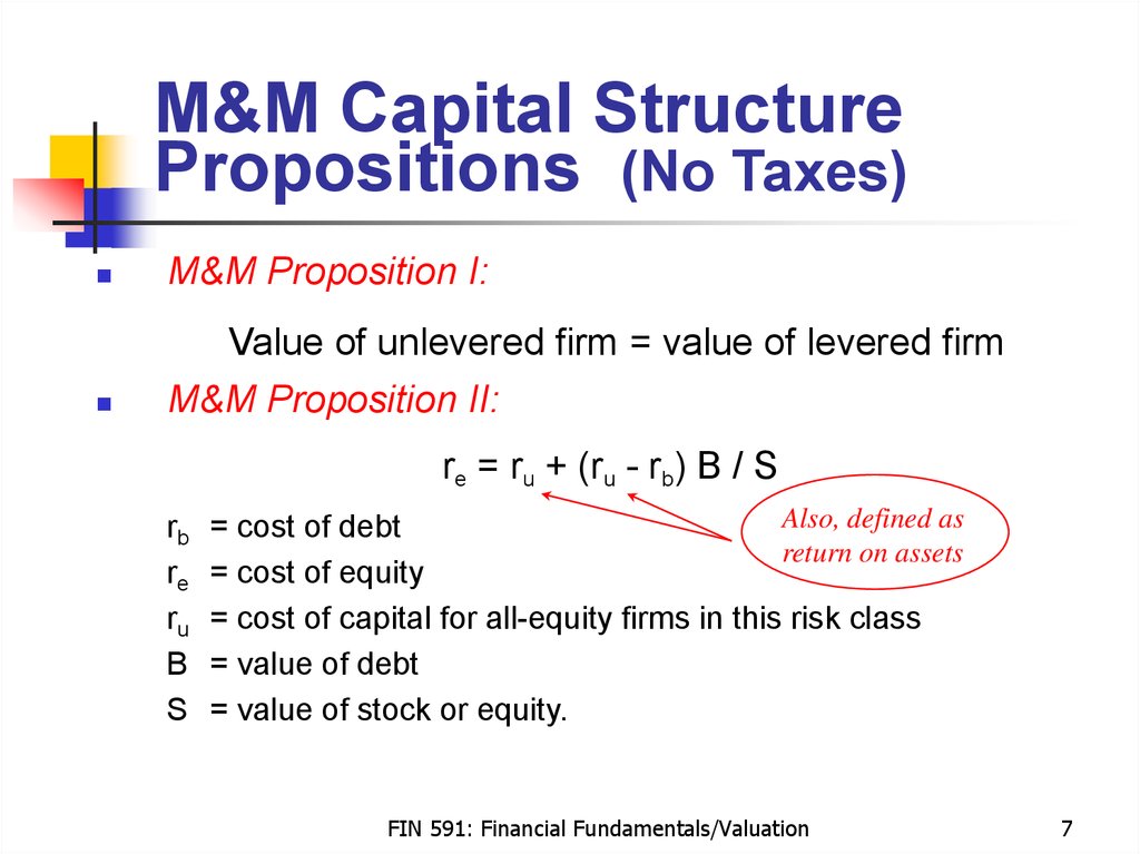
7. M&M Capital Structure Propositions (No Taxes)
M&M Capital StructurePropositions (No Taxes)
M&M Proposition I:
Value of unlevered firm = value of levered firm
M&M Proposition II:
re = ru + (ru - rb) B / S
rb
re
ru
B
S
Also, defined as
= cost of debt
return on assets
= cost of equity
= cost of capital for all-equity firms in this risk class
= value of debt
= value of stock or equity.
FIN 591: Financial Fundamentals/Valuation
7
8. M&M Propositions I & II (No Taxes)
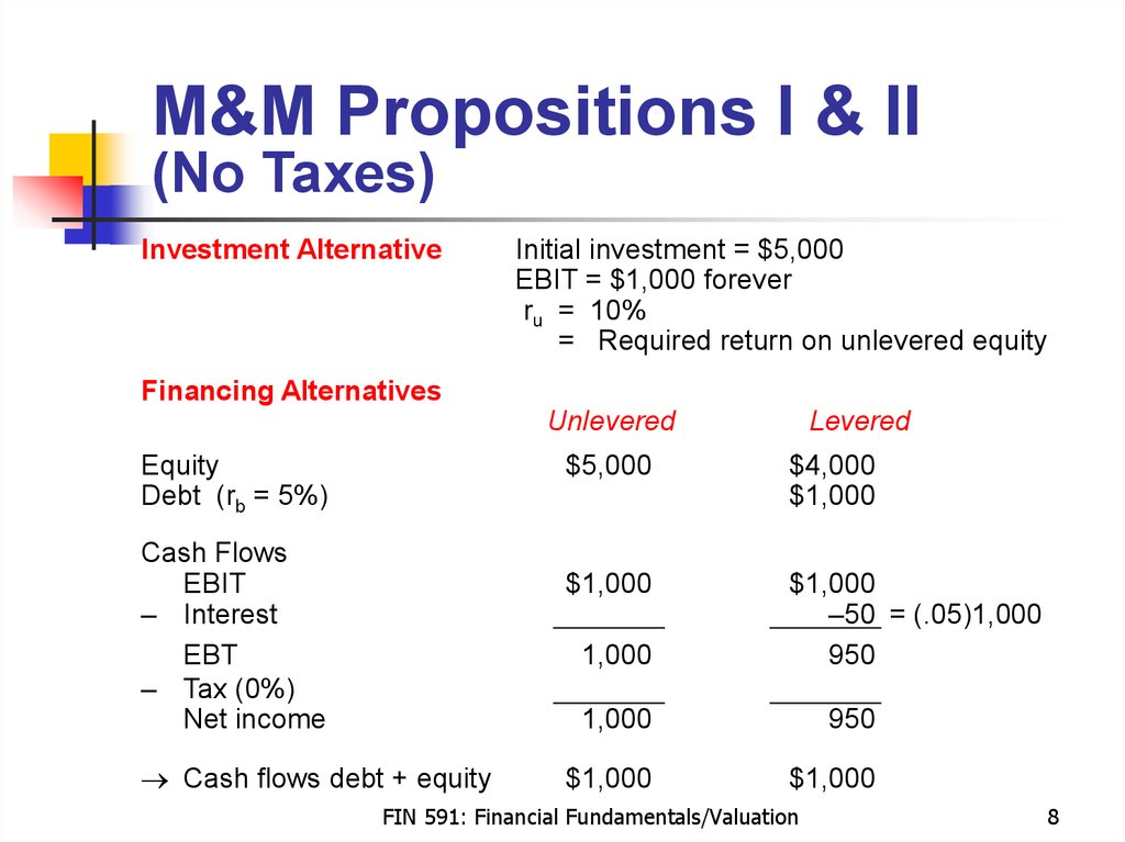
M&M Propositions I & II(No Taxes)
Investment Alternative
Initial investment = $5,000
EBIT = $1,000 forever
ru = 10%
= Required return on unlevered equity
Financing Alternatives
Unlevered
Equity
Debt (rb = 5%)
Cash Flows
EBIT
– Interest
EBT
– Tax (0%)
Net income
$5,000
$4,000
$1,000
$1,000
$1,000
–50 = (.05)1,000
950
1,000
Cash flows debt + equity
Levered
1,000
950
$1,000
$1,000
FIN 591: Financial Fundamentals/Valuation
8
9. M&M Propositions I & II (No Taxes)
M&M Propositions I & II(No Taxes)
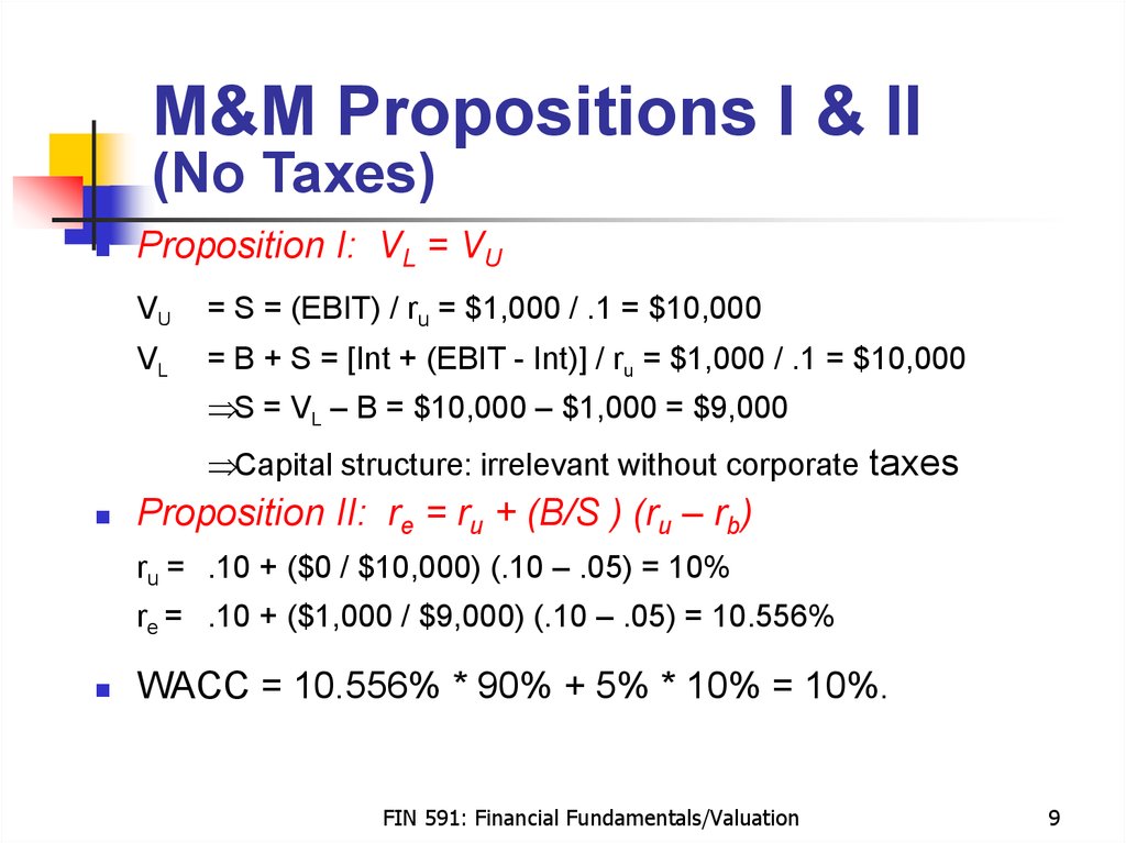
Proposition I: VL = VU
VU
= S = (EBIT) / ru = $1,000 / .1 = $10,000
VL
= B + S = [Int + (EBIT - Int)] / ru = $1,000 / .1 = $10,000
S = VL – B = $10,000 – $1,000 = $9,000
Capital structure: irrelevant without corporate taxes
Proposition II: re = ru + (B/S ) (ru – rb)
ru = .10 + ($0 / $10,000) (.10 – .05) = 10%
re = .10 + ($1,000 / $9,000) (.10 – .05) = 10.556%
WACC = 10.556% * 90% + 5% * 10% = 10%.
FIN 591: Financial Fundamentals/Valuation
9
10. Graphing the M&M No-Tax Relationships
Graphing the M&M No-TaxRelationships
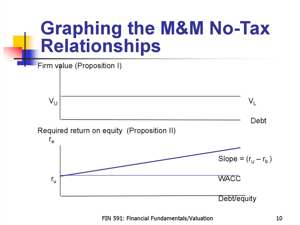
Firm value (Proposition I)
VU
VL
Debt
Required return on equity (Proposition II)
re
Slope = (ru – rb )
ru
WACC
Debt/equity
FIN 591: Financial Fundamentals/Valuation
10
11. M&M Capital Structure Propositions (Corporate Taxes)
M&M Capital StructurePropositions (Corporate Taxes)
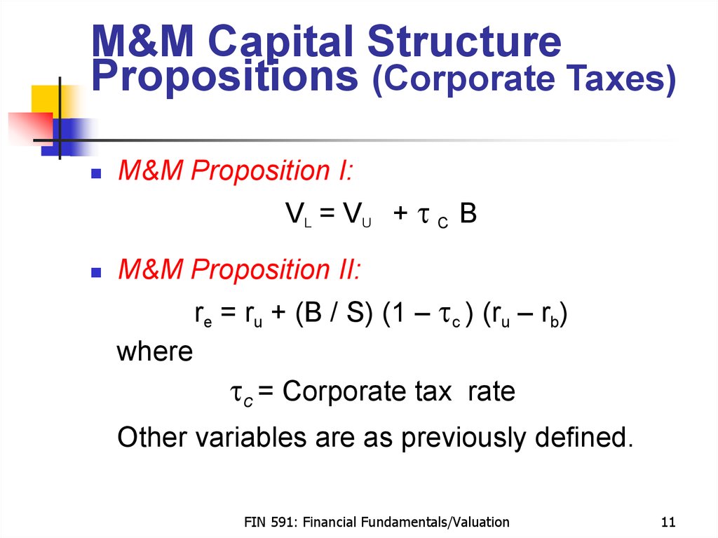
M&M Proposition I:
VL = VU + t C B
M&M Proposition II:
re = ru + (B / S) (1 – tc ) (ru – rb)
where
tc = Corporate tax rate
Other variables are as previously defined.
FIN 591: Financial Fundamentals/Valuation
11
12. M&M Propositions I & II (Corporate Taxes)
M&M Propositions I & II(Corporate Taxes)
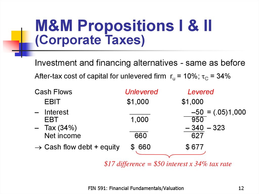
Investment and financing alternatives - same as before
After-tax cost of capital for unlevered firm ru = 10%; tC = 34%
Cash Flows
EBIT
– Interest
EBT
– Tax (34%)
Net income
Unlevered
$1,000
1,000
660
Cash flow debt + equity
Levered
$1,000
–50 = (.05)1,000
950
– 340 – 323
627
$ 660
$ 677
$17 difference = $50 interest x 34% tax rate
FIN 591: Financial Fundamentals/Valuation
12
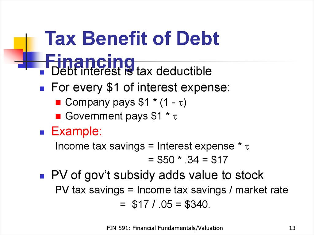
13. Tax Benefit of Debt Financing
Debt interest is tax deductibleFor every $1 of interest expense:
Company pays $1 * (1 - t)
Government pays $1 * t
Example:
Income tax savings = Interest expense * t
= $50 * .34 = $17
PV of gov’t subsidy adds value to stock
PV tax savings = Income tax savings / market rate
= $17 / .05 = $340.
FIN 591: Financial Fundamentals/Valuation
13
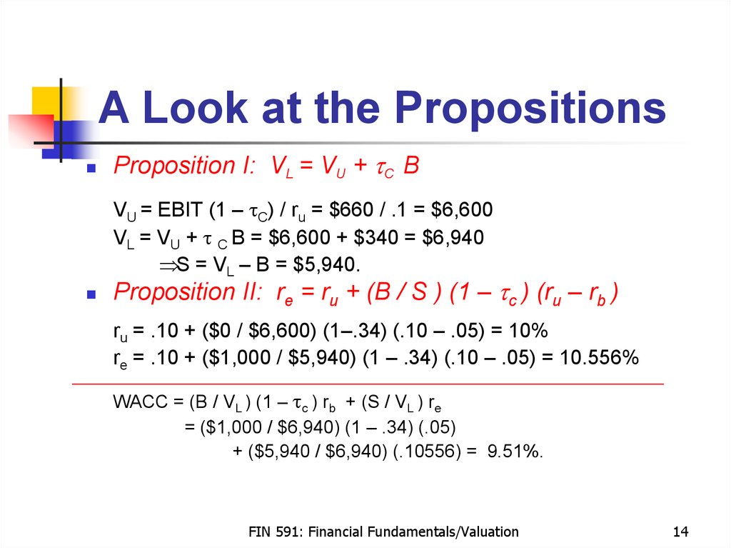
14. A Look at the Propositions
Proposition I: VL = VU + tC BVU = EBIT (1 – tC) / ru = $660 / .1 = $6,600
VL = VU + t C B = $6,600 + $340 = $6,940
S = VL – B = $5,940.
Proposition II: re = ru + (B / S ) (1 – tc ) (ru – rb )
ru = .10 + ($0 / $6,600) (1–.34) (.10 – .05) = 10%
re = .10 + ($1,000 / $5,940) (1 – .34) (.10 – .05) = 10.556%
WACC = (B / VL ) (1 – tc ) rb + (S / VL ) re
= ($1,000 / $6,940) (1 – .34) (.05)
+ ($5,940 / $6,940) (.10556) = 9.51%.
FIN 591: Financial Fundamentals/Valuation
14
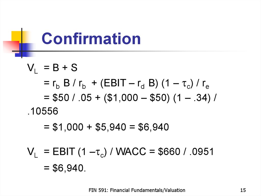
15. Confirmation
VL = B + S= rb B / rb + (EBIT – rd B) (1 – tc) / re
= $50 / .05 + ($1,000 – $50) (1 – .34) /
.10556
= $1,000 + $5,940 = $6,940
VL = EBIT (1 –tc) / WACC = $660 / .0951
= $6,940.
FIN 591: Financial Fundamentals/Valuation
15
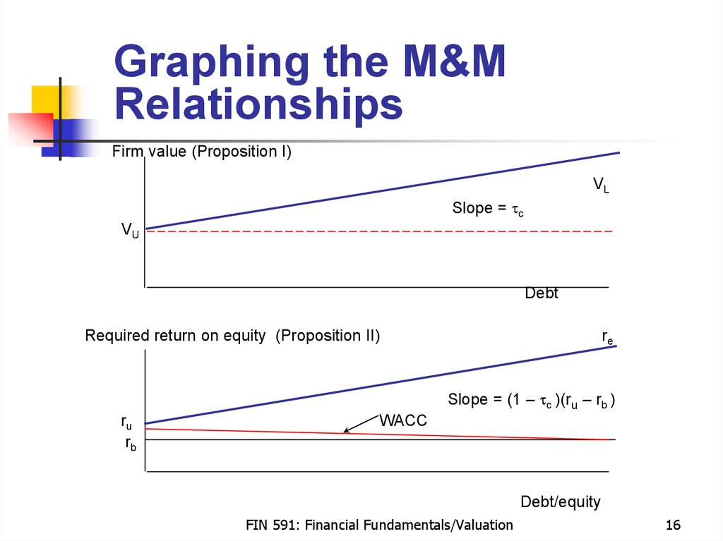
16. Graphing the M&M Relationships
Graphing the M&MRelationships
Firm value (Proposition I)
VL
Slope = tc
VU
Debt
Required return on equity (Proposition II)
re
Slope = (1 – tc )(ru – rb )
ru
rb
WACC
Debt/equity
FIN 591: Financial Fundamentals/Valuation
16
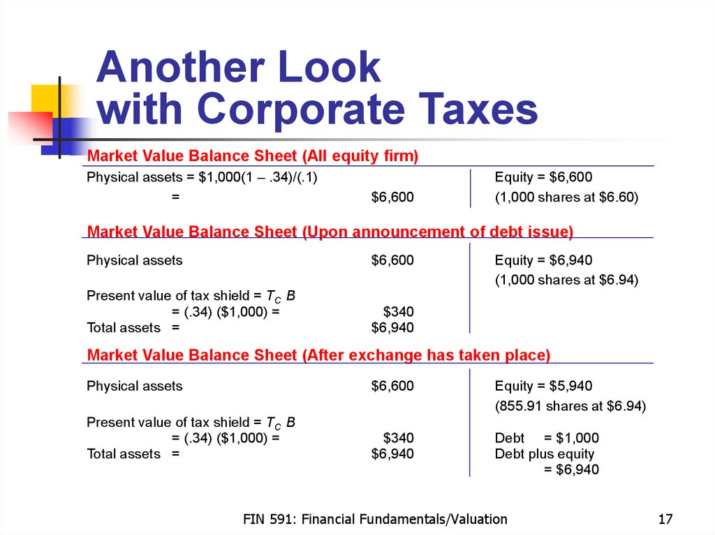
17. Another Look with Corporate Taxes
Market Value Balance Sheet (All equity firm)Physical assets = $1,000(1 – .34)/(.1)
=
$6,600
Equity = $6,600
(1,000 shares at $6.60)
Market Value Balance Sheet (Upon announcement of debt issue)
Physical assets
$6,600
Present value of tax shield = TC B
= (.34) ($1,000) =
Total assets =
$340
$6,940
Equity = $6,940
(1,000 shares at $6.94)
Market Value Balance Sheet (After exchange has taken place)
Physical assets
$6,600
Equity = $5,940
(855.91 shares at $6.94)
Present value of tax shield = TC B
= (.34) ($1,000) =
Total assets =
$340
$6,940
Debt = $1,000
Debt plus equity
= $6,940
FIN 591: Financial Fundamentals/Valuation
17
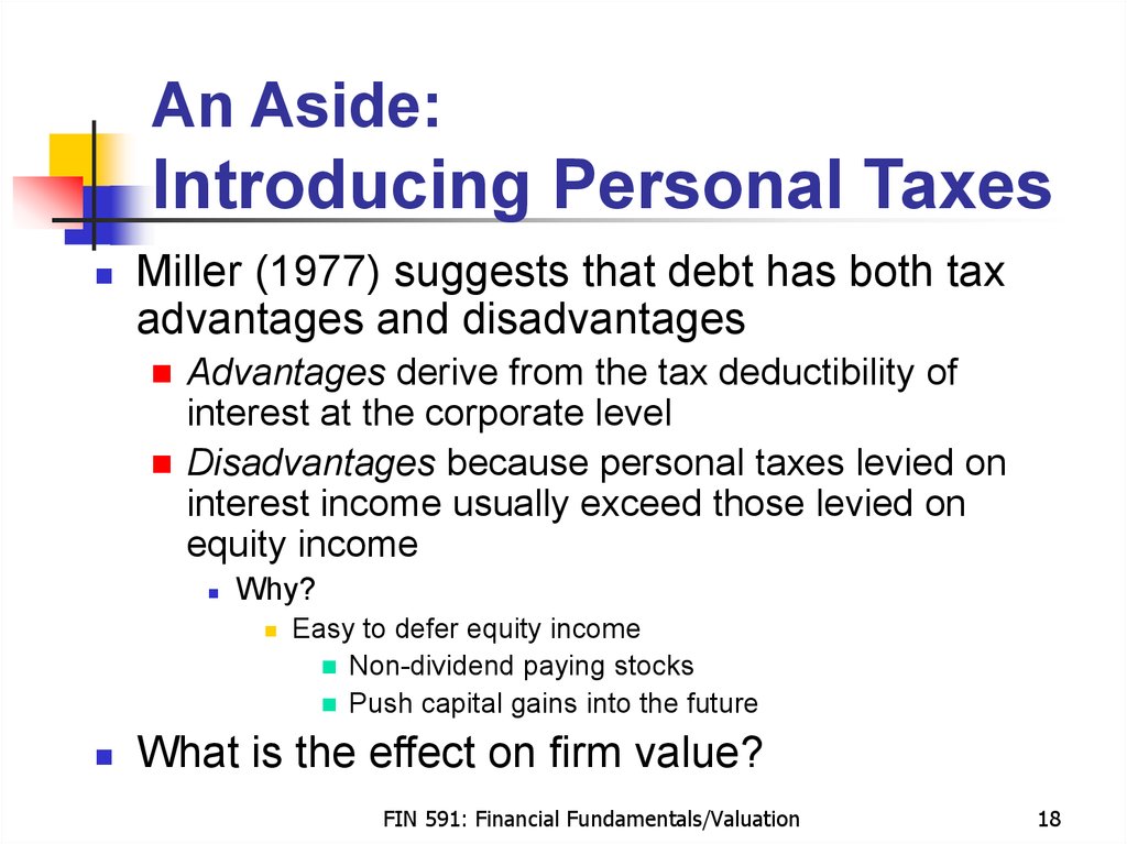
18. An Aside: Introducing Personal Taxes
Miller (1977) suggests that debt has both taxadvantages and disadvantages
Advantages derive from the tax deductibility of
interest at the corporate level
Disadvantages because personal taxes levied on
interest income usually exceed those levied on
equity income
Why?
Easy to defer equity income
Non-dividend paying stocks
Push capital gains into the future
What is the effect on firm value?
FIN 591: Financial Fundamentals/Valuation
18
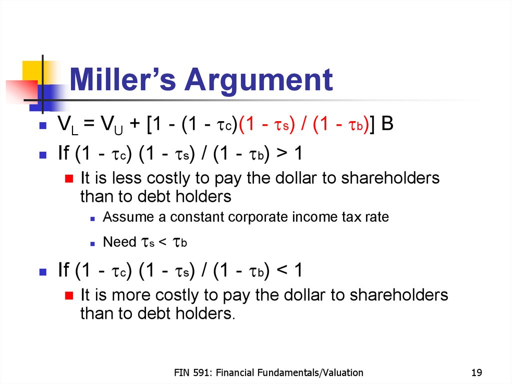
19. Miller’s Argument
VL = VU + [1 - (1 - tc)(1 - ts) / (1 - tb)] BIf (1 - tc) (1 - ts) / (1 - tb) > 1
It is less costly to pay the dollar to shareholders
than to debt holders
tb
If (1 - tc) (1 - ts) / (1 - tb) < 1
Assume a constant corporate income tax rate
Need ts <
It is more costly to pay the dollar to shareholders
than to debt holders.
FIN 591: Financial Fundamentals/Valuation
19
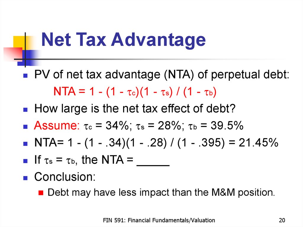
20. Net Tax Advantage
PV of net tax advantage (NTA) of perpetual debt:NTA = 1 - (1 - tc)(1 - ts) / (1 - tb)
How large is the net tax effect of debt?
Assume: tc = 34%; ts = 28%; tb = 39.5%
NTA= 1 - (1 - .34)(1 - .28) / (1 - .395) = 21.45%
If ts = tb, the NTA = _____
Conclusion:
Debt may have less impact than the M&M position.
FIN 591: Financial Fundamentals/Valuation
20
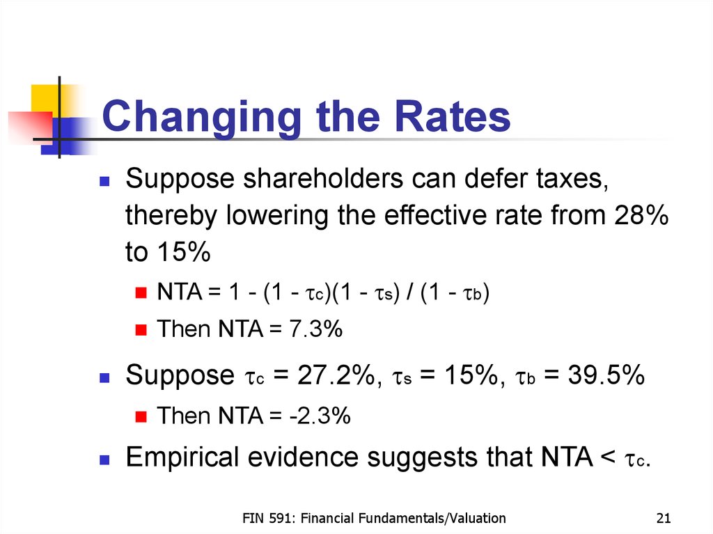
21. Changing the Rates
Suppose shareholders can defer taxes,thereby lowering the effective rate from 28%
to 15%
NTA = 1 - (1 - tc)(1 - ts) / (1 - tb)
Then NTA = 7.3%
Suppose tc = 27.2%, ts = 15%, tb = 39.5%
Then NTA = -2.3%
Empirical evidence suggests that NTA < tc.
FIN 591: Financial Fundamentals/Valuation
21
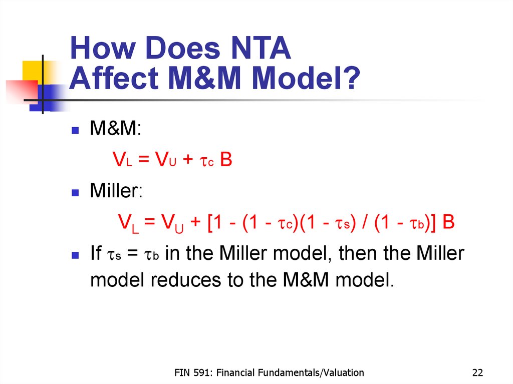
22. How Does NTA Affect M&M Model?
How Does NTAAffect M&M Model?
M&M:
VL = VU + tc B
Miller:
VL = VU + [1 - (1 - tc)(1 - ts) / (1 - tb)] B
If ts = tb in the Miller model, then the Miller
model reduces to the M&M model.
FIN 591: Financial Fundamentals/Valuation
22
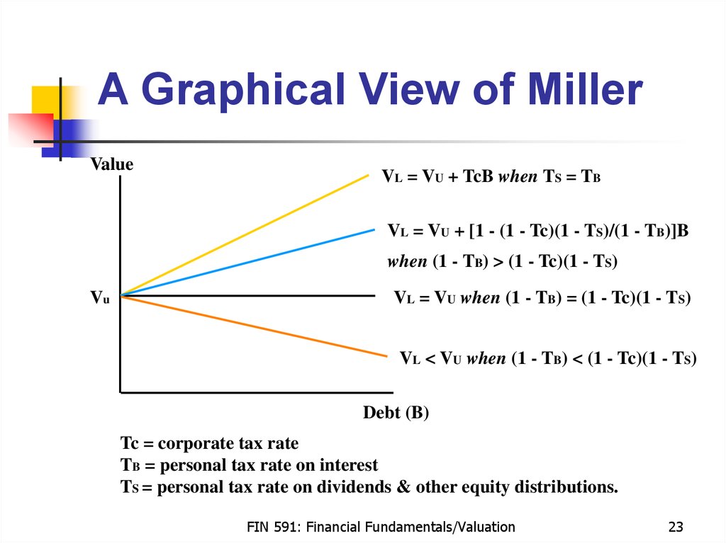
23. A Graphical View of Miller
ValueVL = VU + TcB when TS = TB
VL = VU + [1 - (1 - Tc)(1 - TS)/(1 - TB)]B
when (1 - TB) > (1 - Tc)(1 - TS)
Vu
VL = VU when (1 - TB) = (1 - Tc)(1 - TS)
VL < VU when (1 - TB) < (1 - Tc)(1 - TS)
Debt (B)
Tc = corporate tax rate
TB = personal tax rate on interest
TS = personal tax rate on dividends & other equity distributions.
FIN 591: Financial Fundamentals/Valuation
23
24. Relationship Between Firm Value and WACC
Value of firm = Value of debt + value of equityD(Value) / D(Investment)
= Marginal cost of capital to maintain firm value
DV / DI = ru (1 - tcdB / dI) = WACC
See slide #14
WACC = ru (1 - tc B / S)
= .10 (1 - .34 * 1000 / 6940) = 9.51%
Assumes
ts = tb
Derive WACC from firm value — not vice versa
Earnings perspective
Financing perspective.
FIN 591: Financial Fundamentals/Valuation
24
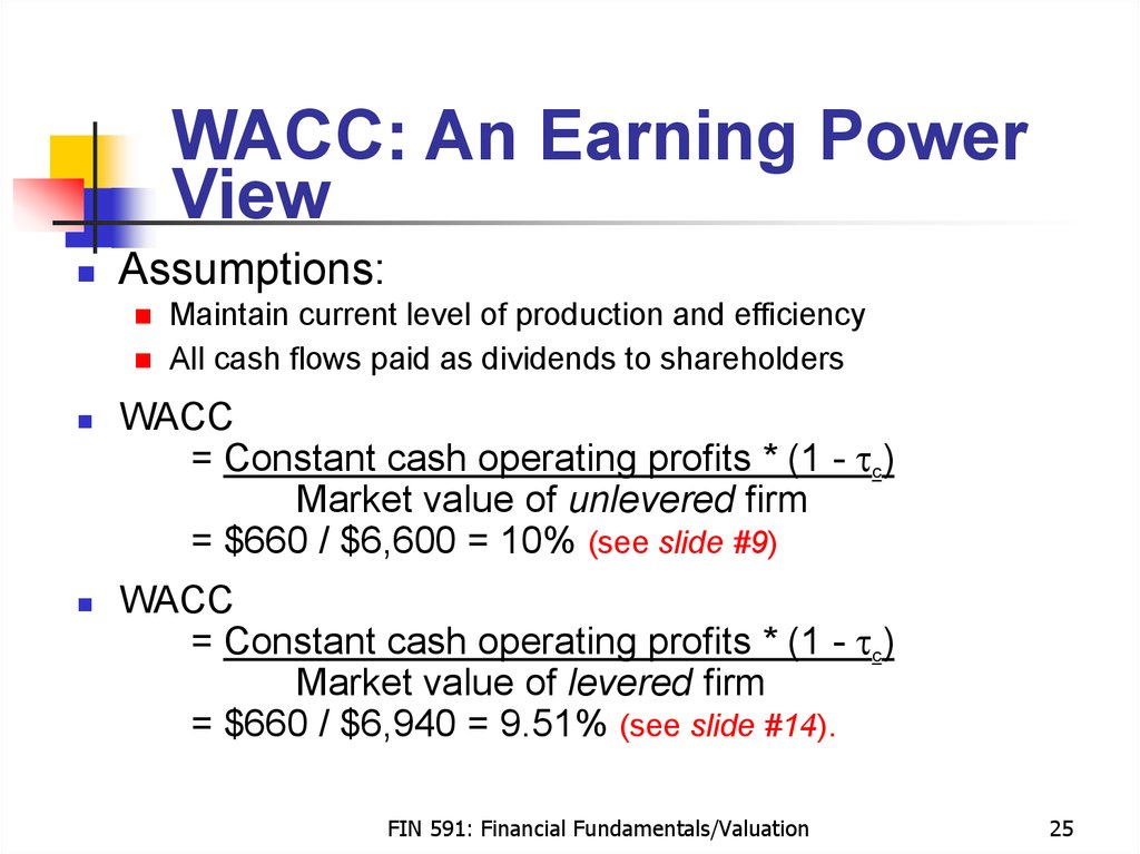
25. WACC: An Earning Power View
Assumptions:Maintain current level of production and efficiency
All cash flows paid as dividends to shareholders
WACC
= Constant cash operating profits * (1 - tc)
Market value of unlevered firm
= $660 / $6,600 = 10% (see slide #9)
WACC
= Constant cash operating profits * (1 - tc)
Market value of levered firm
= $660 / $6,940 = 9.51% (see slide #14).
FIN 591: Financial Fundamentals/Valuation
25
26. WACC: A Financing View
Calculate the cost of:Debt
Preferred stock
Common stock
Combine the different forms of capital into a
weighted average cost of capital — WACC.
FIN 591: Financial Fundamentals/Valuation
26
27. Debt’s Yield to Maturity
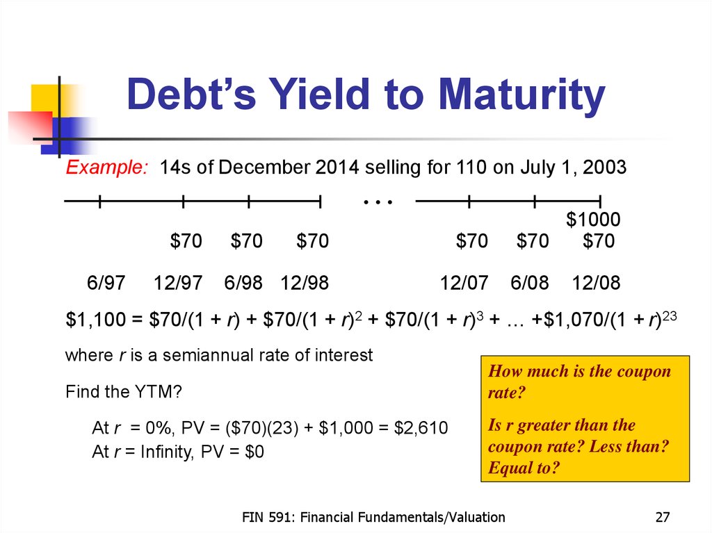
Example: 14s of December 2014 selling for 110 on July 1, 2003...
$70
6/97
12/97
$70
$70
$70
6/98 12/98
12/07
$1000
$70
$70
6/08
12/08
$1,100 = $70/(1 + r) + $70/(1 + r)2 + $70/(1 + r)3 + … +$1,070/(1 + r)23
where r is a semiannual rate of interest
Find the YTM?
At r = 0%, PV = ($70)(23) + $1,000 = $2,610
At r = Infinity, PV = $0
How much is the coupon
rate?
Is r greater than the
coupon rate? Less than?
Equal to?
FIN 591: Financial Fundamentals/Valuation
27
28. A Graphical View: YTM
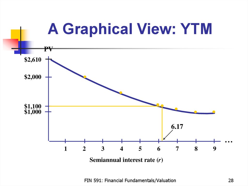
PV$2,610
$2,000
$1,100
$1,000
6.17
…
1
2
3
4
5
6
7
8
9
Semiannual interest rate (r)
FIN 591: Financial Fundamentals/Valuation
28
29. Cost of Debt
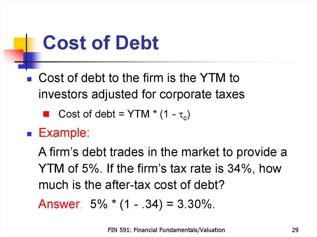
Cost of debt to the firm is the YTM toinvestors adjusted for corporate taxes
Cost of debt = YTM * (1 - tc)
Example:
A firm’s debt trades in the market to provide a
YTM of 5%. If the firm’s tax rate is 34%, how
much is the after-tax cost of debt?
Answer: 5% * (1 - .34) = 3.30%.
FIN 591: Financial Fundamentals/Valuation
29
30. Cost of Debt = YTM * (1 - tc)
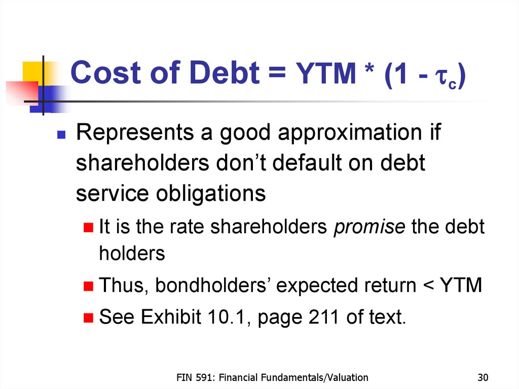
Represents a good approximation ifshareholders don’t default on debt
service obligations
It
is the rate shareholders promise the debt
holders
Thus,
See
bondholders’ expected return < YTM
Exhibit 10.1, page 211 of text.
FIN 591: Financial Fundamentals/Valuation
30
31. Cost of Preferred Stock
Preferred stock dividend is not tax deductibleCost is the market return earned by investors:
Dividend / market price of preferred stock
Example:
A preferred stock (par = $20) pays a $3
dividend annually. It currently trades in the
market for $24. How much is the cost of the
stock from the firm’s perspective?
Answer: $3 / $24 = 12.5%.
FIN 591: Financial Fundamentals/Valuation
31
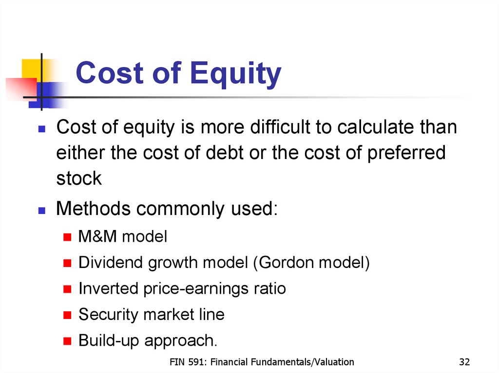
32. Cost of Equity
Cost of equity is more difficult to calculate thaneither the cost of debt or the cost of preferred
stock
Methods commonly used:
M&M model
Dividend growth model (Gordon model)
Inverted price-earnings ratio
Security market line
Build-up approach.
FIN 591: Financial Fundamentals/Valuation
32
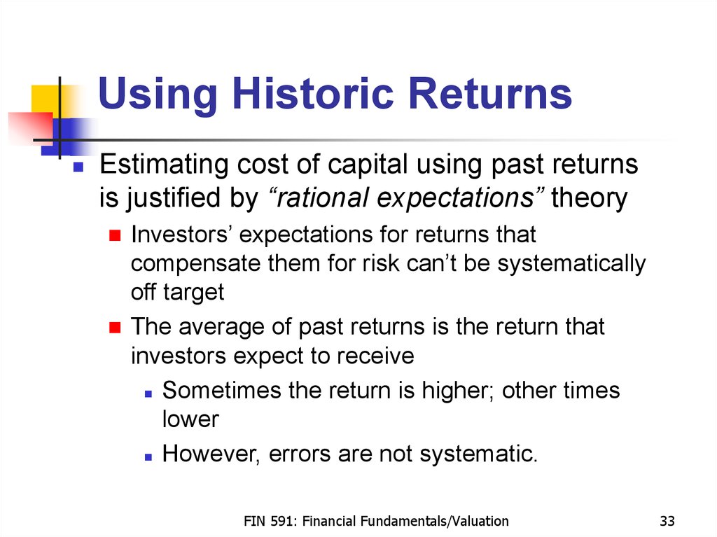
33. Using Historic Returns
Estimating cost of capital using past returnsis justified by “rational expectations” theory
Investors’ expectations for returns that
compensate them for risk can’t be systematically
off target
The average of past returns is the return that
investors expect to receive
Sometimes the return is higher; other times
lower
However, errors are not systematic.
FIN 591: Financial Fundamentals/Valuation
33
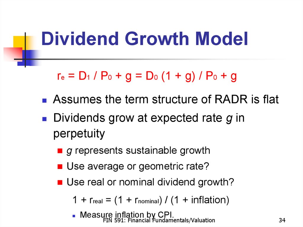
34. Dividend Growth Model
re = D1 / P0 + g = D0 (1 + g) / P0 + gAssumes the term structure of RADR is flat
Dividends grow at expected rate g in
perpetuity
g represents sustainable growth
Use average or geometric rate?
Use real or nominal dividend growth?
1 + rreal = (1 + rnominal) / (1 + inflation)
Measure inflation by CPI.
FIN 591: Financial Fundamentals/Valuation
34
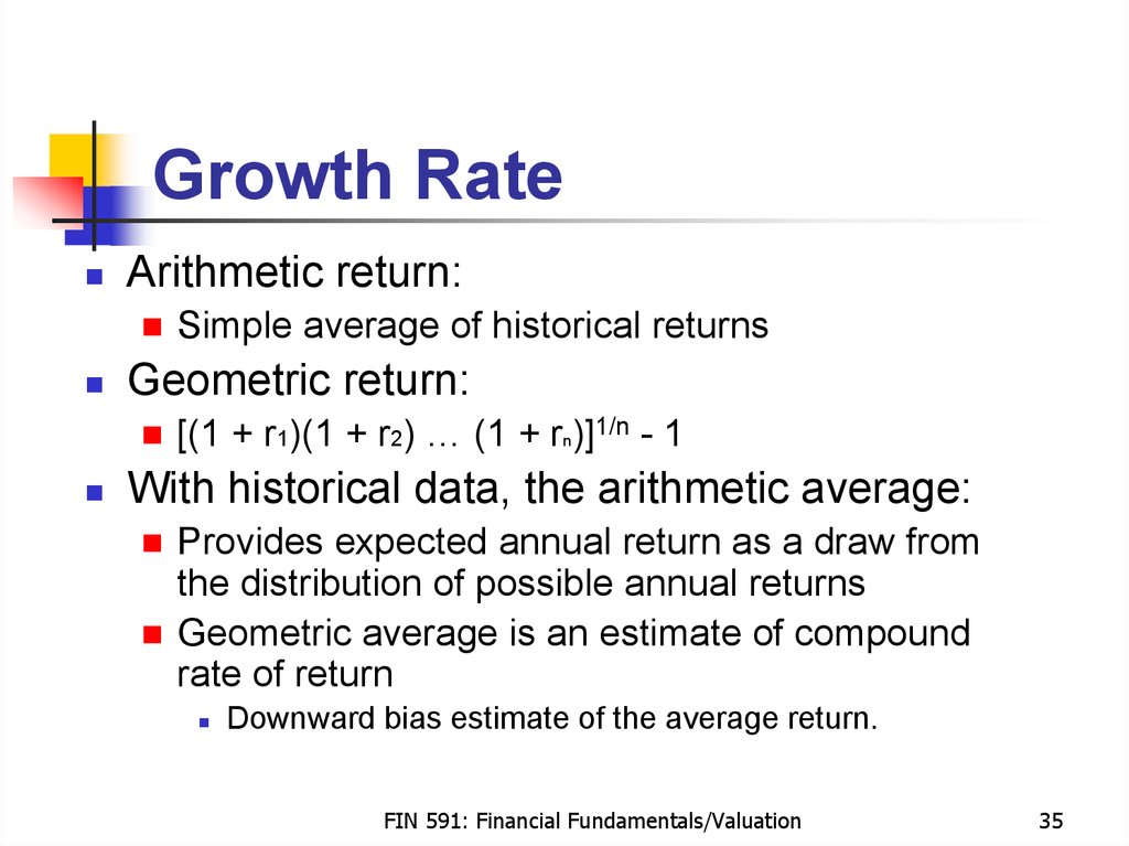
35. Growth Rate
Arithmetic return:Geometric return:
Simple average of historical returns
[(1 + r1)(1 + r2) … (1 + rn)]1/n - 1
With historical data, the arithmetic average:
Provides expected annual return as a draw from
the distribution of possible annual returns
Geometric average is an estimate of compound
rate of return
Downward bias estimate of the average return.
FIN 591: Financial Fundamentals/Valuation
35
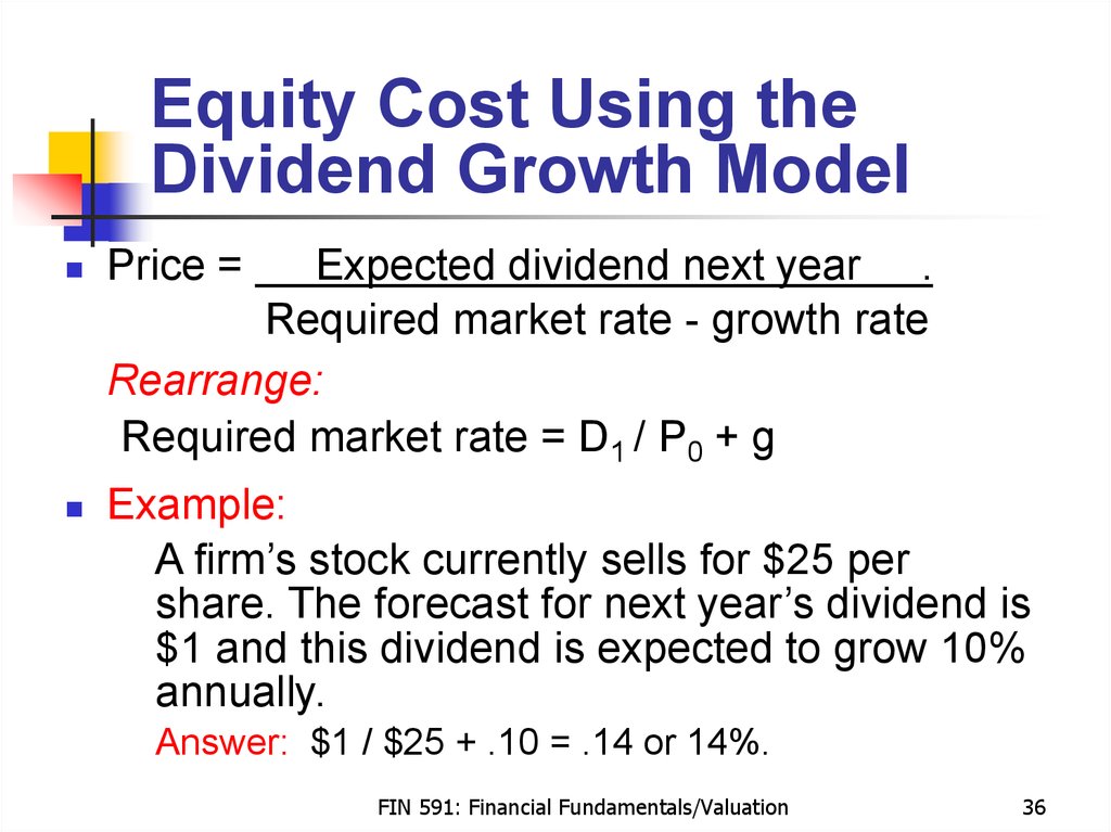
36. Equity Cost Using the Dividend Growth Model
Price =Expected dividend next year .
Required market rate - growth rate
Rearrange:
Required market rate = D1 / P0 + g
Example:
A firm’s stock currently sells for $25 per
share. The forecast for next year’s dividend is
$1 and this dividend is expected to grow 10%
annually.
Answer: $1 / $25 + .10 = .14 or 14%.
FIN 591: Financial Fundamentals/Valuation
36
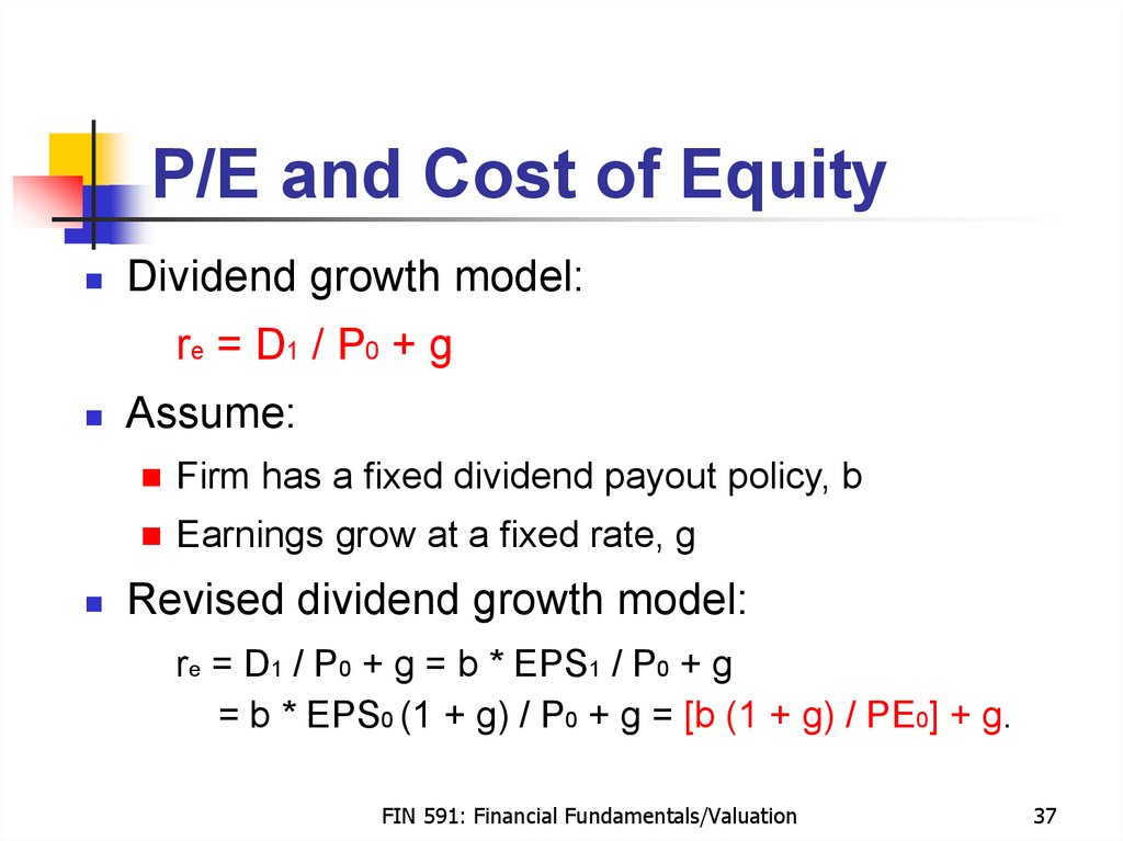
37. P/E and Cost of Equity
Dividend growth model:re = D1 / P0 + g
Assume:
Firm has a fixed dividend payout policy, b
Earnings grow at a fixed rate, g
Revised dividend growth model:
re = D1 / P0 + g = b * EPS1 / P0 + g
= b * EPS0 (1 + g) / P0 + g = [b (1 + g) / PE0] + g.
FIN 591: Financial Fundamentals/Valuation
37
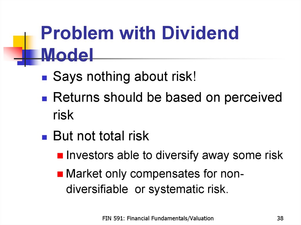
38. Problem with Dividend Model
Says nothing about risk!Returns should be based on perceived
risk
But not total risk
Investors
able to diversify away some risk
Market
only compensates for nondiversifiable or systematic risk.
FIN 591: Financial Fundamentals/Valuation
38
39. The End
FIN 591: Financial Fundamentals/Valuation39



 Английский язык


