Factor Models: Announcements, Surprises, and Expected Returns

1.

11.1 Factor Models: Announcements, Surprises, and
Expected Returns
11.2 Risk: Systematic and Unsystematic
11.3 Systematic Risk and Betas
11.4 Portfolios and Factor Models
11.5 Betas and Expected Returns
11.6 The Capital Asset Pricing Model and the Arbitrage
Pricing Theory
11.7 Parametric Approaches to Asset Pricing
11.8 Summary and Conclusions

2. 11.1 Factor Models: Announcements, Surprises, and Expected Returns

• The return on any security consists of two parts.
1) the expected or normal return: the return that
shareholders in the market predict or expect
2) the unexpected or risky return: the portion that comes
from information that will be revealed .
Examples of relevant information:
– Statistics Canada figures (e.g., GNP)
– A sudden drop in interest rates
– News that the company’s sales figures are higher than
expected

3. 11.1 Factor Models: Announcements, Surprises, and Expected Returns

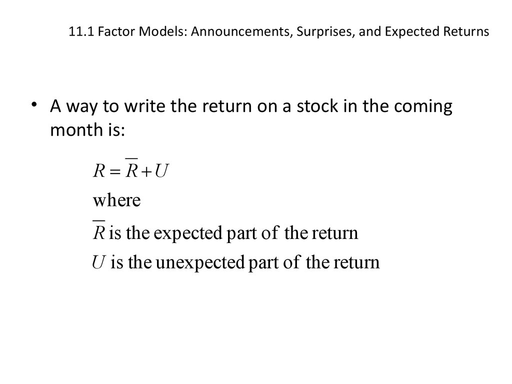
• A way to write the return on a stock in the coming
month is:
R R U
where
R is the expected part of the return
U is the unexpected part of the return

4. 11.1 Factor Models: Announcements, Surprises, and Expected Returns

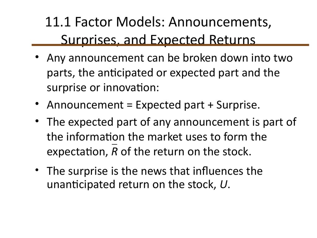
• Any announcement can be broken down into two
parts, the anticipated or expected part and the
surprise or innovation:
• Announcement = Expected part + Surprise.
• The expected part of any announcement is part of
the information the market uses to form the
expectation, R of the return on the stock.
• The surprise is the news that influences the
unanticipated return on the stock, U.

5. 11.2 Risk: Systematic and Unsystematic

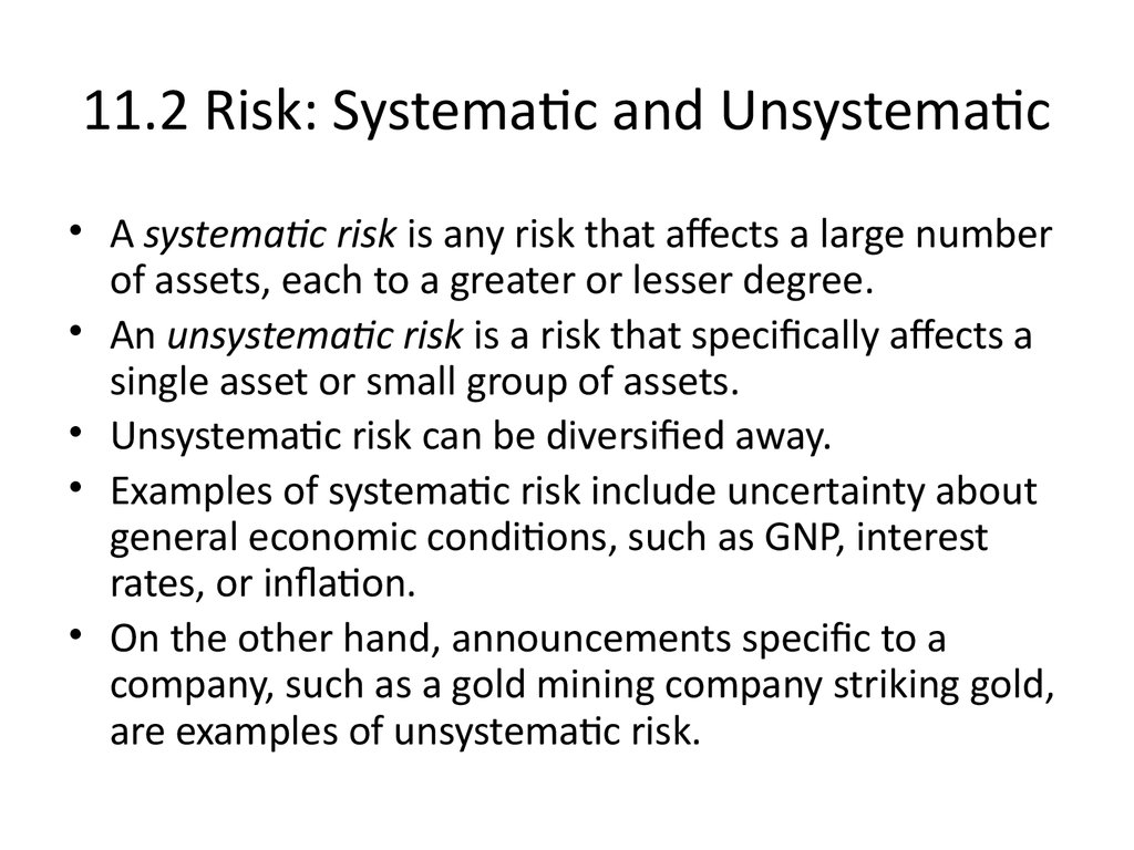
• A systematic risk is any risk that affects a large number
of assets, each to a greater or lesser degree.
• An unsystematic risk is a risk that specifically affects a
single asset or small group of assets.
• Unsystematic risk can be diversified away.
• Examples of systematic risk include uncertainty about
general economic conditions, such as GNP, interest
rates, or inflation.
• On the other hand, announcements specific to a
company, such as a gold mining company striking gold,
are examples of unsystematic risk.

6. 11.2 Risk: Systematic and Unsystematic

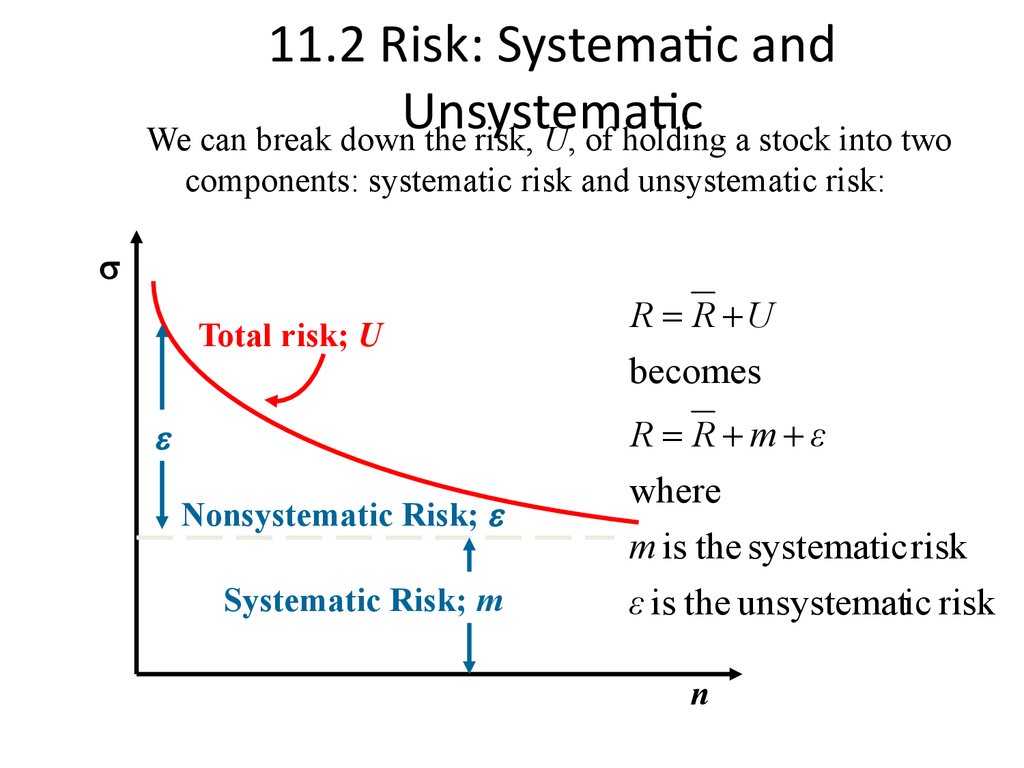
We can break down the risk, U, of holding a stock into two
components: systematic risk and unsystematic risk:
Total risk; U
R R U
becomes
R R m ε
Nonsystematic Risk;
Systematic Risk; m
where
m is the systematic risk
ε is the unsystematic risk
n

7. 11.2 Risk: Systematic and Unsystematic

Systematic risk is referred to as market risk.
m influences all assets in the market to some extent.
ε
Is specific to the company and unrelated to the
specific risk of most other companies.
Corr ( ε ε ) 0
i,
j

8. 11.3 Systematic Risk and Betas

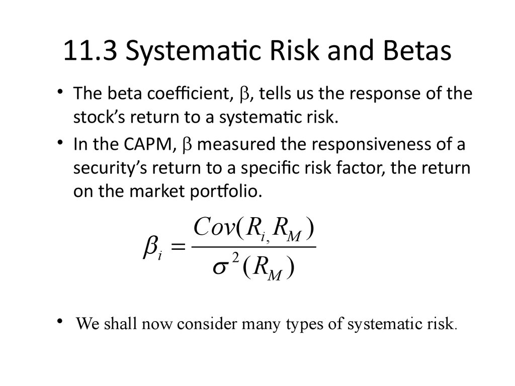
• The beta coefficient, b, tells us the response of the
stock’s return to a systematic risk.
• In the CAPM, b measured the responsiveness of a
security’s return to a specific risk factor, the return
on the market portfolio.
bi
Cov( Ri , RM )
( RM )
2
• We shall now consider many types of systematic risk.

9. 11.3 Systematic Risk and Betas

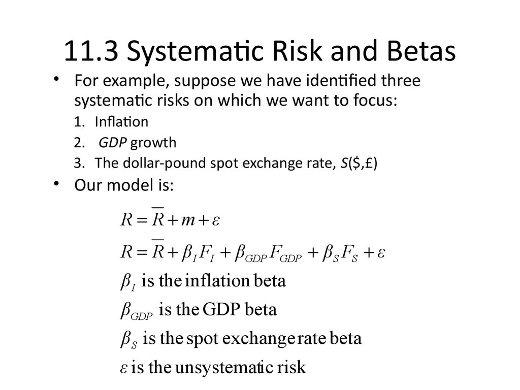
• For example, suppose we have identified three
systematic risks on which we want to focus:
1. Inflation
2. GDP growth
3. The dollar-pound spot exchange rate, S($,£)
• Our model is:
R R m ε
R R β I FI βGDP FGDP βS FS ε
β I is the inflation beta
βGDP is the GDP beta
βS is the spot exchange rate beta
ε is the unsystematic risk

10. Systematic Risk and Betas: Example

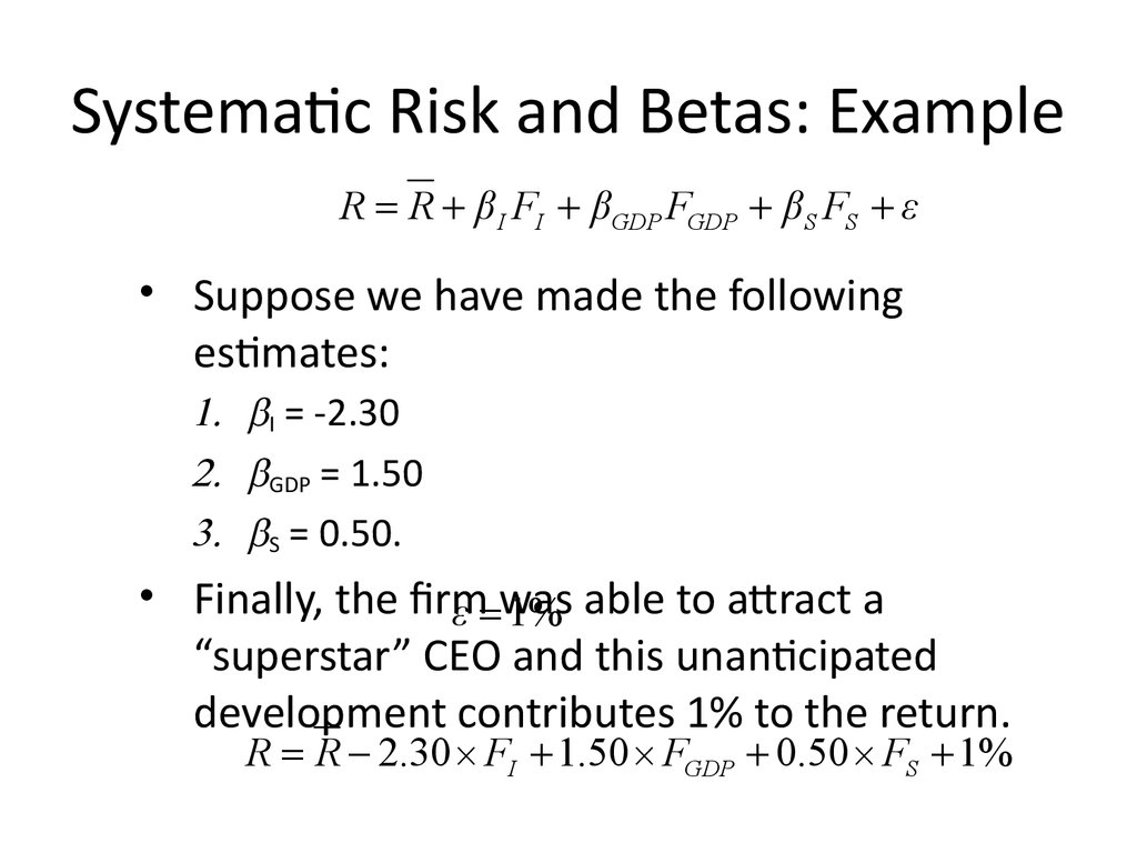
R R βI FI βGDP FGDP βS FS ε
• Suppose we have made the following
estimates:
1. bI = -2.30
2. bGDP = 1.50
3. bS = 0.50.
• Finally, the firm
ε was
1% able to attract a
“superstar” CEO and this unanticipated
development contributes 1% to the return.
R R 2.30 FI 1.50 FGDP 0.50 FS 1%

11. Systematic Risk and Betas: Example

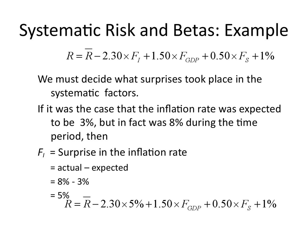
R R 2.30 FI 1.50 FGDP 0.50 FS 1%
We must decide what surprises took place in the
systematic factors.
If it was the case that the inflation rate was expected
to be 3%, but in fact was 8% during the time
period, then
FI = Surprise in the inflation rate
= actual – expected
= 8% - 3%
= 5%
R R 2.30 5% 1.50 FGDP 0.50 FS 1%

12. Systematic Risk and Betas: Example

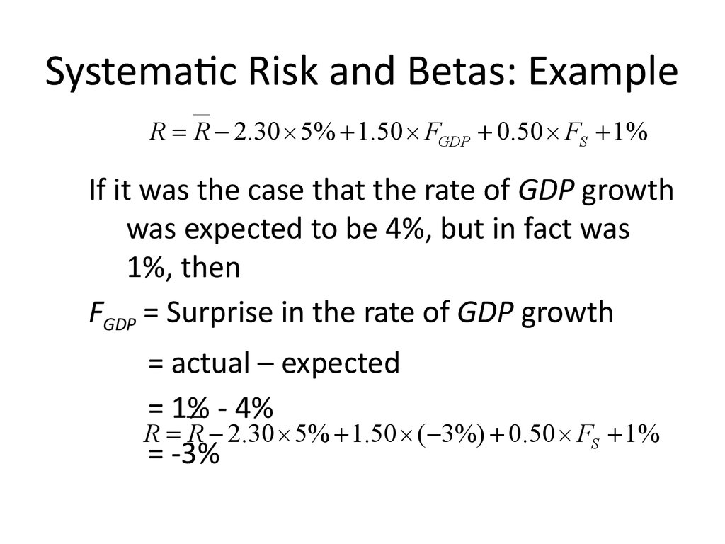
R R 2.30 5% 1.50 FGDP 0.50 FS 1%
If it was the case that the rate of GDP growth
was expected to be 4%, but in fact was
1%, then
FGDP = Surprise in the rate of GDP growth
= actual – expected
= 1% - 4%
R R 2.30 5% 1.50 ( 3%) 0.50 FS 1%
= -3%

13. Systematic Risk and Betas: Example

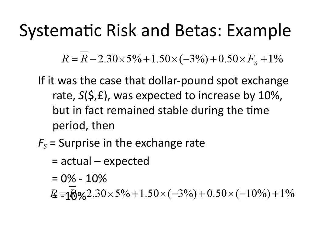
R R 2.30 5% 1.50 ( 3%) 0.50 FS 1%
If it was the case that dollar-pound spot exchange
rate, S($,£), was expected to increase by 10%,
but in fact remained stable during the time
period, then
FS = Surprise in the exchange rate
= actual – expected
= 0% - 10%
R= -10%
R 2.30 5% 1.50 ( 3%) 0.50 ( 10%) 1%

14. Systematic Risk and Betas: Example

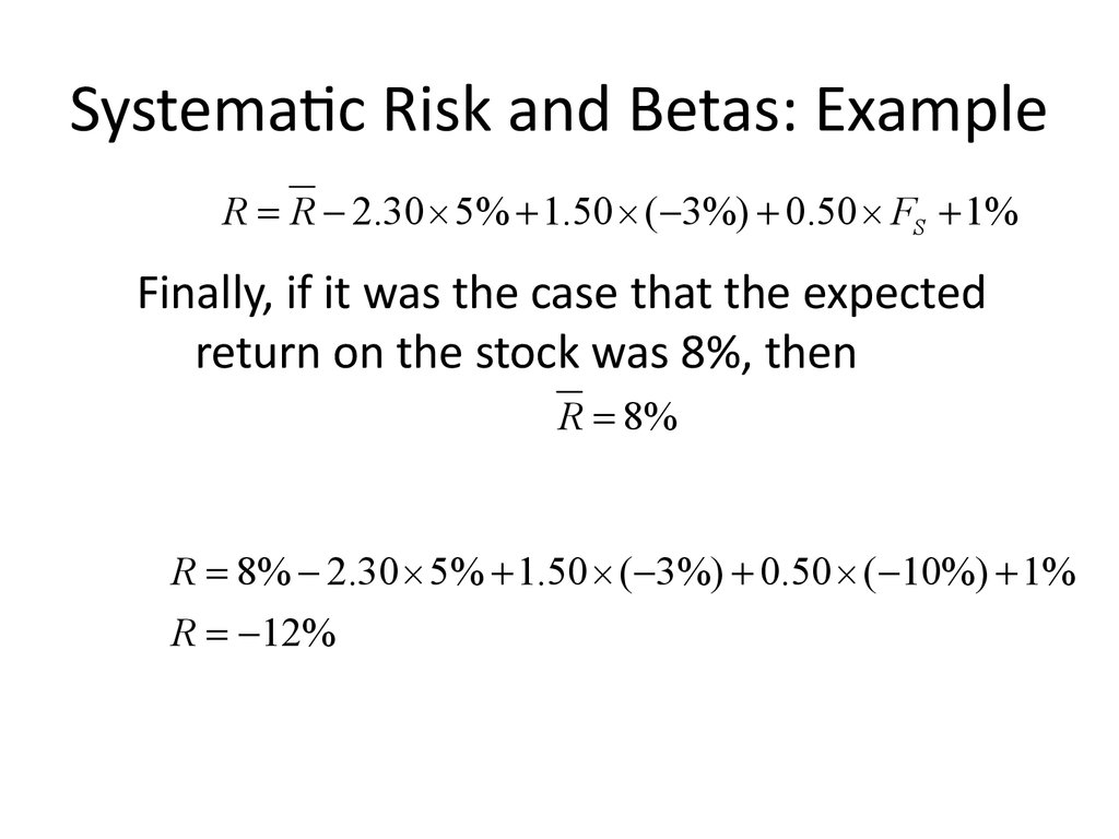
R R 2.30 5% 1.50 ( 3%) 0.50 FS 1%
Finally, if it was the case that the expected
return on the stock was 8%, then
R 8%
R 8% 2.30 5% 1.50 ( 3%) 0.50 ( 10%) 1%
R 12%

15. 11.4 Portfolios and Factor Models

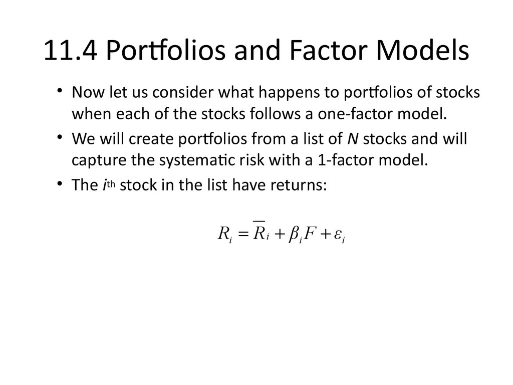
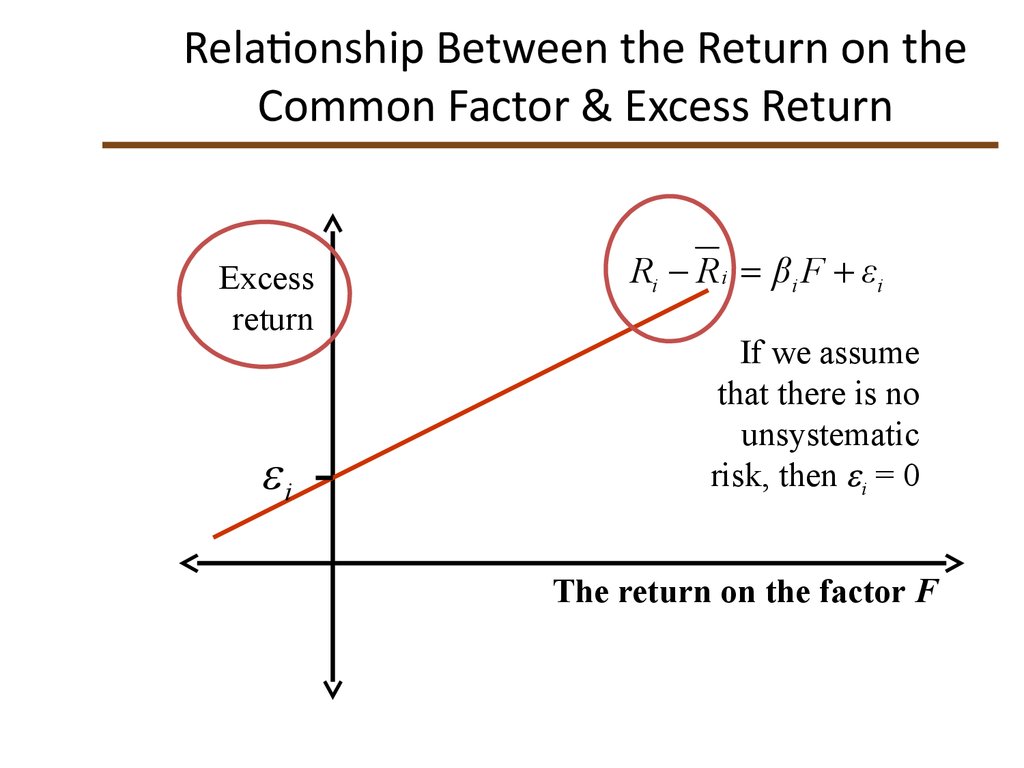
• Now let us consider what happens to portfolios of stocks
when each of the stocks follows a one-factor model.
• We will create portfolios from a list of N stocks and will
capture the systematic risk with a 1-factor model.
• The ith stock in the list have returns:
Ri R i βi F εi

16. Relationship Between the Return on the Common Factor & Excess Return

Relationship Between the Return on the
Common Factor & Excess Return
Excess
return
i
Ri R i βi F εi
If we assume
that there is no
unsystematic
risk, then i = 0
The return on the factor F

17. Relationship Between the Return on the Common Factor & Excess Return

Relationship Between the Return on the
Common Factor & Excess Return
Excess
return
Ri R i βi F
If we assume
that there is no
unsystematic
risk, then i = 0
The return on the factor F

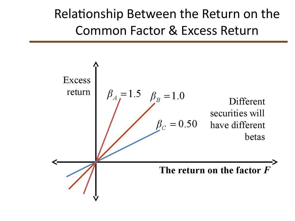
18. Relationship Between the Return on the Common Factor & Excess Return

Relationship Between the Return on the
Common Factor & Excess Return
Excess
return
β A 1.5 β B 1.0
βC 0.50
Different
securities will
have different
betas
The return on the factor F

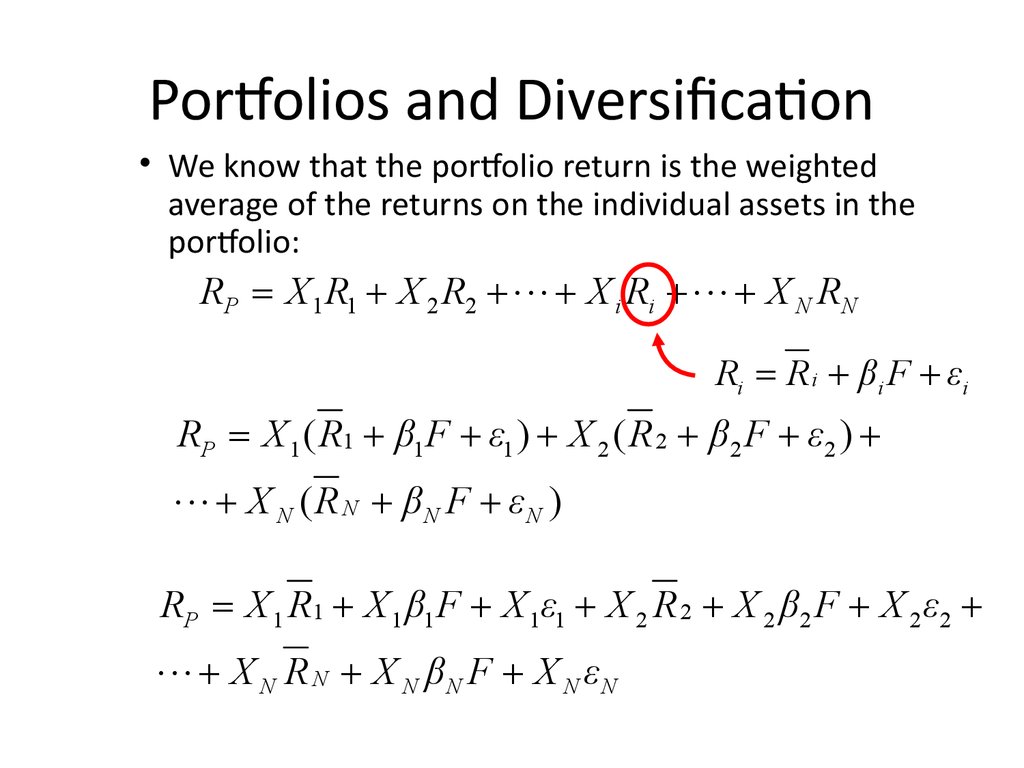
19. Portfolios and Diversification

• We know that the portfolio return is the weighted
average of the returns on the individual assets in the
portfolio:
RP X 1 R1 X 2 R2 X i Ri X N RN
Ri R i βi F εi
RP X 1 ( R1 β1 F ε1 ) X 2 ( R 2 β2 F ε2 )
X N ( R N βN F εN )
RP X 1 R1 X 1 β1 F X 1ε1 X 2 R 2 X 2 β2 F X 2 ε2
X N R N X N βN F X N εN

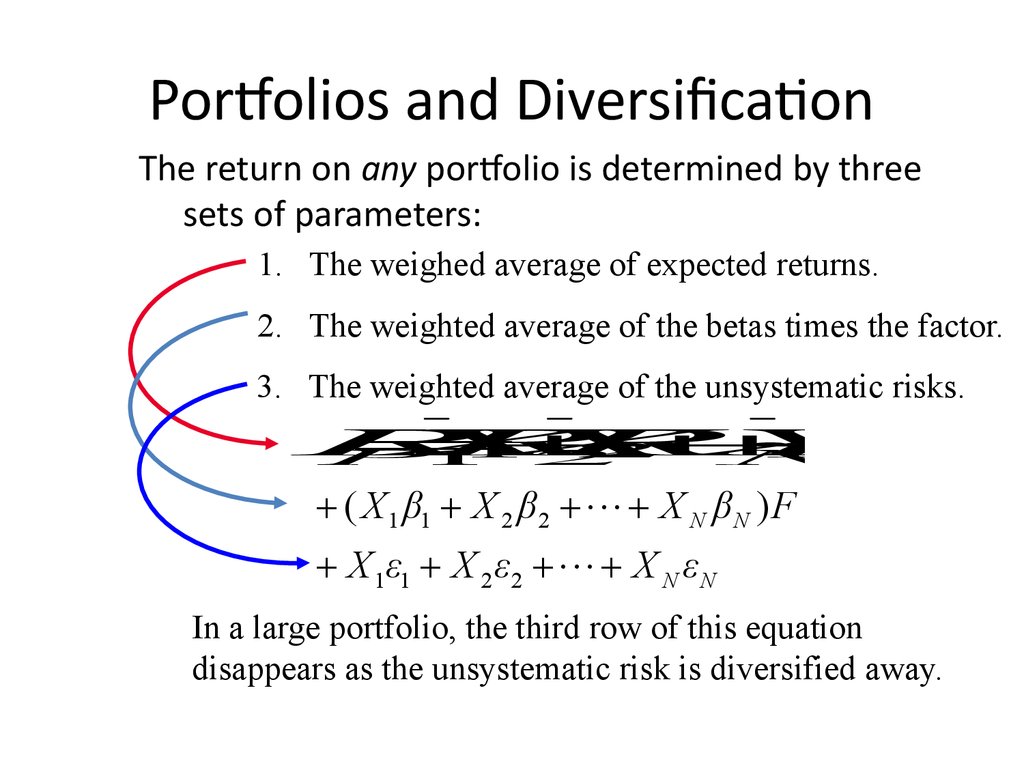
20. Portfolios and Diversification

The return on any portfolio is determined by three
sets of parameters:
1. The weighed average of expected returns.
2. The weighted average of the betas times the factor.
3. The weighted average of the unsystematic risks.
R
X
R
X
R
X
R
1
2
N
P
1
2
N
( X 1 β1 X 2 β2 X N β N ) F
X 1ε1 X 2 ε2 X N ε N
In a large portfolio, the third row of this equation
disappears as the unsystematic risk is diversified away.

21. Portfolios and Diversification

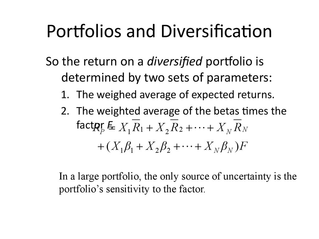
So the return on a diversified portfolio is
determined by two sets of parameters:
1. The weighed average of expected returns.
2. The weighted average of the betas times the
factor
RP F. X 1 R1 X 2 R 2 X N R N
( X 1 β1 X 2 β2 X N β N ) F
In a large portfolio, the only source of uncertainty is the
portfolio’s sensitivity to the factor.

22. 11.5 Betas and Expected Returns

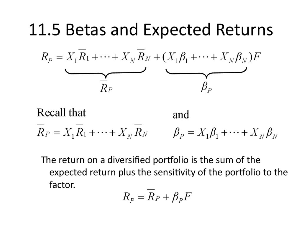
RP X 1 R1 X N R N ( X 1 β1 X N β N ) F
βP
RP
Recall that
and
R P X 1 R1 X N R N
β P X 1 β1 X N β N
The return on a diversified portfolio is the sum of the
expected return plus the sensitivity of the portfolio to the
factor.
RP R P βP F

23. Relationship Between b & Expected Return

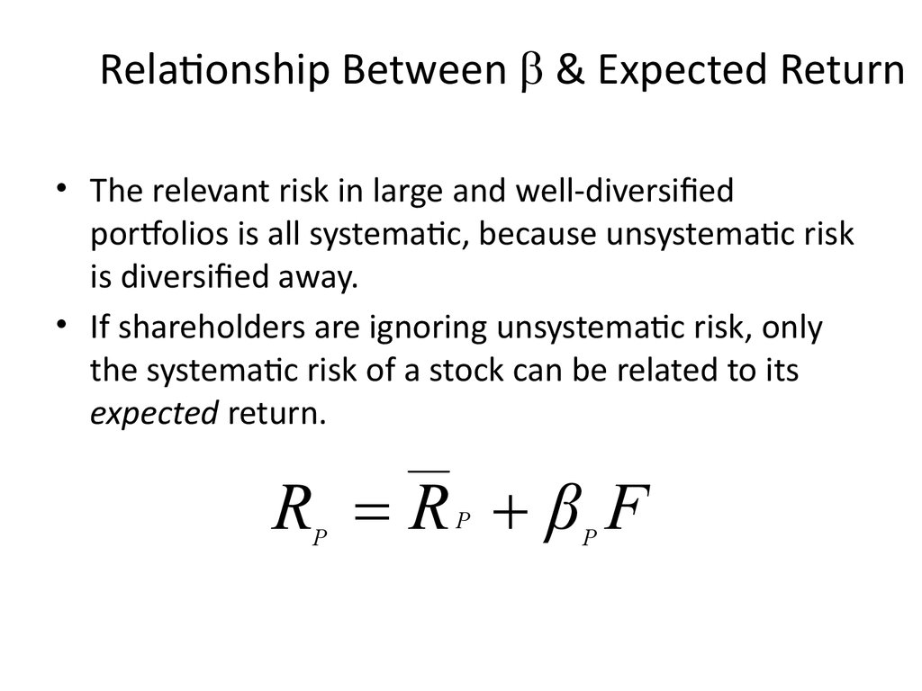
Relationship Between b & Expected Return
• The relevant risk in large and well-diversified
portfolios is all systematic, because unsystematic risk
is diversified away.
• If shareholders are ignoring unsystematic risk, only
the systematic risk of a stock can be related to its
expected return.
R R β F
P
P
P

24. Relationship Between b & Expected Return

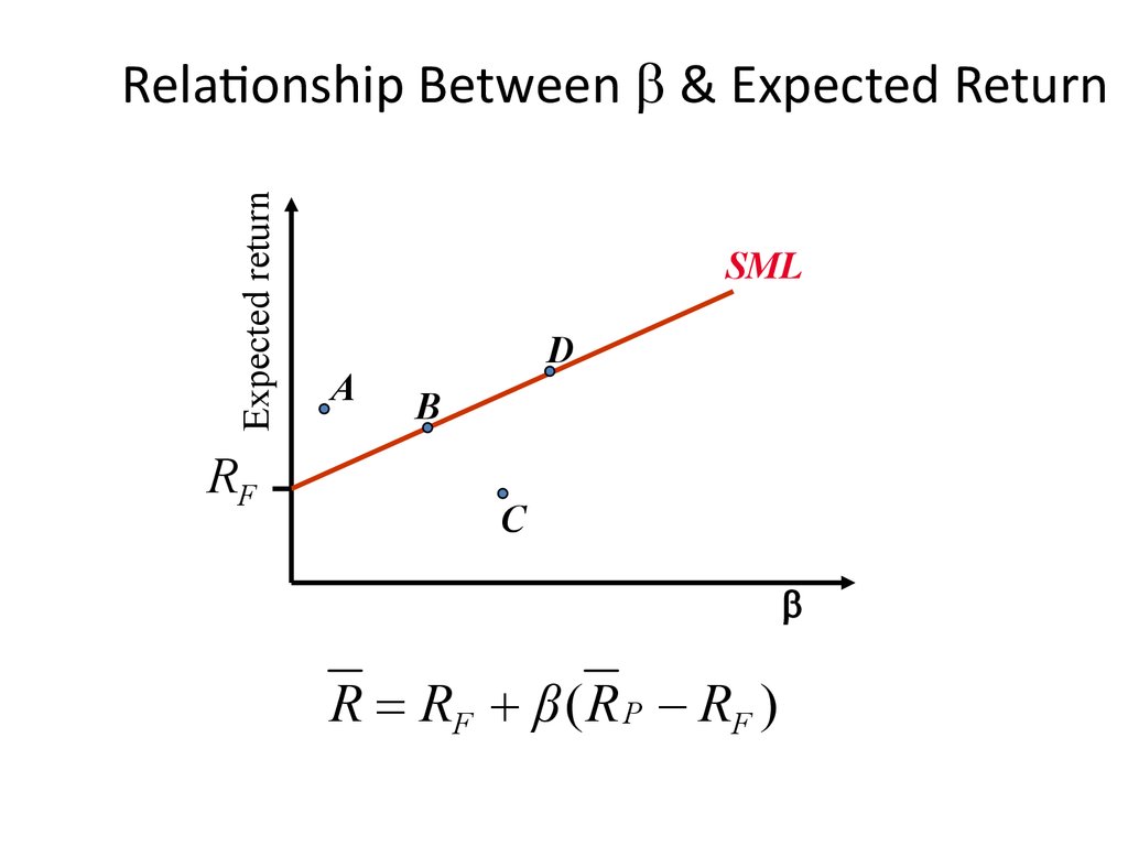
Expected return
Relationship Between b & Expected Return
RF
SML
A
D
B
C
b
R RF β ( R P RF )

25. 11.6 The Capital Asset Pricing Model and the Arbitrage Pricing Theory

• APT applies to well diversified portfolios and not
necessarily to individual stocks.
• With APT it is possible for some individual stocks to
be mispriced---not lie on the SML.
• APT is more general in that it gets to an expected
return and beta relationship without the assumption
of the market portfolio.
• APT can be extended to multifactor models.

26. Multi-factor APT

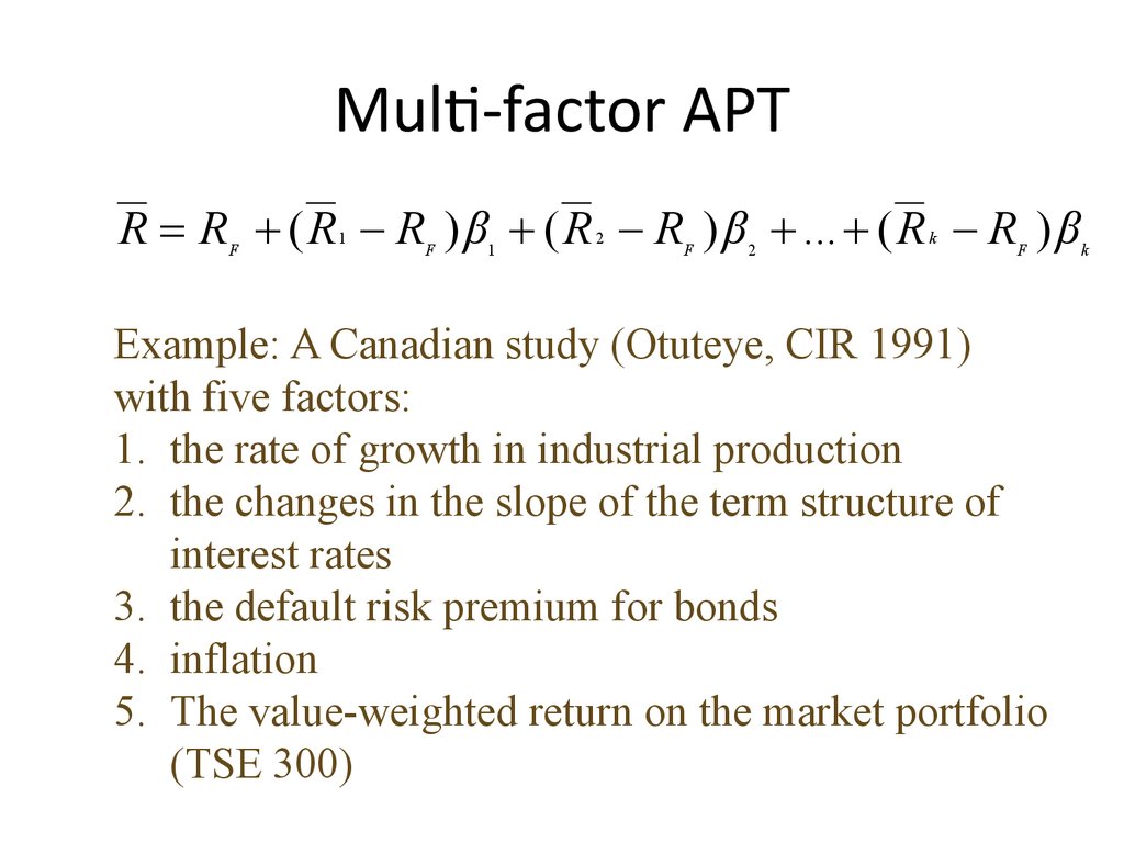
R R ( R R ) β ( R R ) β ... ( R R ) β
F
1
F
1
2
F
2
k
F
Example: A Canadian study (Otuteye, CIR 1991)
with five factors:
1. the rate of growth in industrial production
2. the changes in the slope of the term structure of
interest rates
3. the default risk premium for bonds
4. inflation
5. The value-weighted return on the market portfolio
(TSE 300)
k

27. 11.7 Empirical Approaches to Asset Pricing

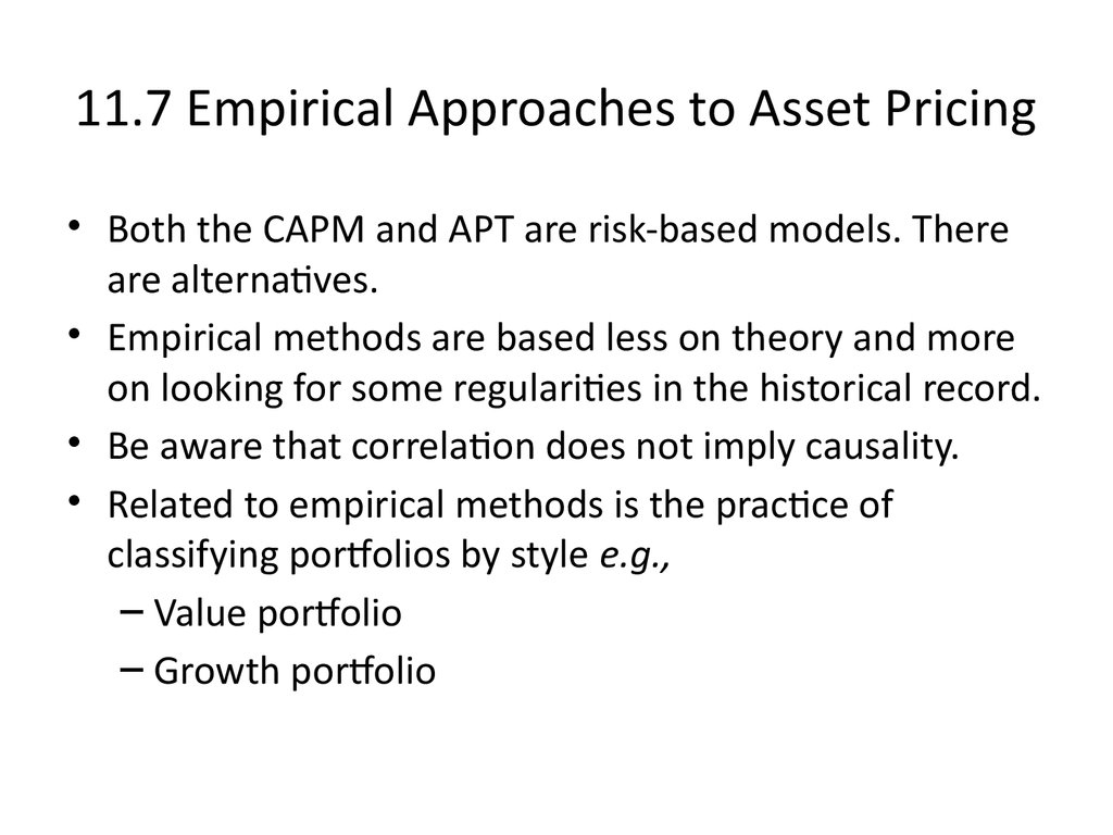
• Both the CAPM and APT are risk-based models. There
are alternatives.
• Empirical methods are based less on theory and more
on looking for some regularities in the historical record.
• Be aware that correlation does not imply causality.
• Related to empirical methods is the practice of
classifying portfolios by style e.g.,
– Value portfolio
– Growth portfolio

28. 11.8 Summary and Conclusions

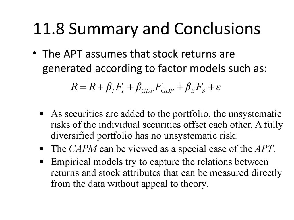
• The APT assumes that stock returns are
generated according to factor models such as:
R R βI FI βGDP FGDP βS FS ε
· As securities are added to the portfolio, the unsystematic
risks of the individual securities offset each other. A fully
diversified portfolio has no unsystematic risk.
· The CAPM can be viewed as a special case of the APT.
· Empirical models try to capture the relations between
returns and stock attributes that can be measured directly
from the data without appeal to theory.